JSON Code

//////////////////////////////////////////////////////

JSON

______________________________________________________

maXbox Starter 82 -JSON in Code – Max Kleiner

“There is always space for improvement”

— Oscar De La Hoya

mX4

JSON (JavaScript Object Notation) is a lightweight data-interchange format. It is easy for humans to read and write. It is easy for machines to parse and generate. A JSON Parser is then used to format the JSON data into a properly readable JSON Format with curly brackets. That can easily view and identify its key and values.

{

“date”: “2021-3-4”,

“confirmed”: 36223,

“deaths”: 1483,

“recovered”: 33632

}

Reading JSON data in maXbox could be easy. Json data can be read from a file or it could be a json web link. Let us first try to read the json from a web link.

Const

JsonUrl = ‘https://pomber.github.io/covid19/timeseries.json’;

We use JSON for Delphi framework (json4delphi), it supports older versions of Delphi and Lazarus (6 or above) and is very versatile. Another advantage is the Objectpascal native code, using classes only TList, TStrings, TStringStream, TCollection and TStringList; The package contains 3 units: Jsons.pas, JsonsUtilsEx.pas and a project Testunit, available at: https://github.com/rilyu/json4delphi

Now we need a Load URL or Upload File function to get the json data for parsing. In our case load is a function-pair of open and send().

Let us first define the necessary packages “msxml2.xmlhttp” and the JSON class itself:

var XMLhttp: OleVariant; // As Object Automation

ajt: TJson; JObj: TJsonObject2;

XMLhttp:= CreateOleObject(‘msxml2.xmlhttp’)

XMLhttp.Open(‘GET’, JsonUrl, False) //False is async

XMLhttp.setRequestHeader(‘Content-Type’,’application/x-www-form-urlencoded’);

XMLhttp.Send();

response:= XMLhttp.responseText; //assign the data

statuscode:= XMLhttp.status;

Using async = false in Open() is not always recommended, but for a few small requests this can be ok. Remember that the script will NOT continue to execute, until the server response is ready. If the server is busy or slow, the application will hang or stop.

Anyway we open our XMLhttpObject (which is late binding) as not asynchronous, that is to say, synchronous because we need all data to continue:

Ref: <class ‘pandas.core.frame.DataFrame’>

RangeIndex: 76608 entries, 0 to 76607

Data columns (total 5 columns):

# Column Non-Null Count Dtype

— —— ————– —–

0 country 76608 non-null object

1 date 76608 non-null object

2 confirmed 76608 non-null int64

3 deaths 76608 non-null int64

4 recovered 76608 non-null int64

dtypes: int64(3), object(2)

memory usage: 2.9+ MB

Worldwide Covid Deaths: 2517422 at the end of Feb. 2021

The send() method (XMLhttp.Send();) needs a further explanation: send() accepts an optional parameter which lets you specify the requests body; this is primarily used for requests such as PUT or POST. If the request method is GET or HEAD, the body parameter is ignored and the request body is set to null.

I’m not sure if the content-type is the right, the MIME media type for JSON text is application/json and the default encoding is UTF-8. (Source: RFC 4627).

{content-type: application/json; charset=utf-8}

JSON is a SUB-TYPE of text but not text alone. Json is a text representation of an object (or array of objects). So I think both should be allowed. The question is which works better in practice and solution.

By the way if no Accept header has been set using the setRequestHeader(), an Accept header with the type “*/*” (any type) is sent.

Next we define the Json instance:

ajt:= TJson.create();

For slicing (filter) the data we copy the range from response timeseries.json:

startR:= pos(‘”‘+ACOUNTRY1+'”‘,response);

stopR:= pos(‘”‘+ACOUNTRY2+'”‘,response);

writeln(‘DataLen Overall: ‘+itoa(length(response)))

resrange:= Copy(response, startR, stopR-startR);

resrange:= ‘{‘+resrange+’}’; //well formed

Now we parse the response.

try

ajt.parse(resrange);

except

writeln( ‘Exception: <TJson>”” parse error: {‘+

exceptiontostring(exceptiontype, exceptionparam))

end;

Now we can iterate through the keys with values as items. Here, in the above sample JSON data: date, confirmed, deaths and recovered are known as key and “2020-1-22”, 0, 0 and 0 known as a Value. All Data are available in a Key and value pair.

First we get a list of all 192 country names as the node name:

JObj:= ajt.JsonObject;

writeln(‘Get all Countries: ‘)

for cnt:= 0 to jobj.count-1 do

writeln(Jobj.items[cnt].name);

…United Kingdom

Uruguay

Uzbekistan

Vanuatu

Venezuela

Vietnam…

So the country is an object to get. Ok, it is a JsonObject dictionary with 192 countries. Lets check the keys of our dict with a nested loop of all confirmed cases:

for cnt:= 0 to Jobj.count-1 do begin

Clabel:= Jobj.items[cnt].name;

JArray2:= jobj.values[Clabel].asArray;

for cnt2:= 0 to jarray2.count-1 do

itmp:= jarray2.items[cnt2].asObject.values[‘confirmed’].asinteger;

end;

So we pass the country name items[cnt].name from the Json Object in to the value list and we get back an a object array for the second iteration of at the moment 408 records with key values of integer format. Our dimension for now is 192 * 408 = 78336 records.

<class ‘pandas.core.frame.DataFrame’>

RangeIndex: 78336 entries, 0 to 78335

Data columns (total 5 columns):

# Column Non-Null Count Dtype

— —— ————– —–

0 country 78336 non-null object

1 date 78336 non-null object

2 confirmed 78336 non-null int64

3 deaths 78336 non-null int64

4 recovered 78336 non-null int64

dtypes: int64(3), object(2)

memory usage: 3.0+ MB

{

“Afghanistan”: [

{

“date”: “2020-1-22”,

“confirmed”: 0,

“deaths”: 0,

“recovered”: 0

},

{

“date”: “2020-1-23”,

“confirmed”: 0,

“deaths”: 0,

“recovered”: 0

},…

In a second attempt we visualize the timeseries with TeeChart Standard. Ok we got the objectarray as sort of dataframe with items and values but not in the form that we wanted. We will have to unwind the nested data like above to build a proper dataframe with chart series at runtime for TChart:

Chart1.Title.Text.clear;

//AssignSeries(OldSeries,NewSeries:TChartSeries);

Chart1.Title.Text.add(‘Sciplot Serie: ‘+’World Covid21 confirmed not †’);

Chart1.Axes.Bottom.Title.Caption:= ‘Days from ‘+

datetimetostr(date-400)+’ to ‘+datetimetostr(date-1);

Chart1.BottomAxis.Labels:= True;

Chart1.LeftAxis.Logarithmic:= true;

//Chart1.XValues.Multiplier:= 1

Clabel:=”;

for cnt:= 0 to Jobj.count-1 do begin

Clabel:= Jobj.items[cnt].name

JArray2:= jobj.values[Clabel].asarray;

chart1.AddSeries(TFastLineSeries.Create(Self)); //runtime instances

chart1.series[cnt].title:= Clabel;

TFastLineSeries(chart1.series[cnt]).LinePen.Width:= 4;

for cnt2:= jarray2.count-400 to jarray2.count-1 do begin

itmp:= jarray2.items[cnt2].asObject.values[‘confirmed’].asinteger;

sumup:= sumup+ itmp

chart1.Series[cnt].Addxy(cnt2,itmp, itoa(cnt2),clRed);

end;

end;

writeln(‘Worldwide Count:’+itoa(ajt.count)+’ Covid Confirm: ‘+itoa(sumup));//*)

The plot you can find at:

http://www.softwareschule.ch/examples/covid3.png

TeeChart is a charting library for programmers, developed and managed by Steema Software of Girona, Catalonia, Spain. It is available as commercial and non-commercial software. TeeChart has been included in most Delphi and C++Builder products since 1997, and TeeChart Standard currently is part of Embarcadero RAD Studio 10.4 Sydney.

Conclusion:

The proper way to use JSON is to specify types that must be compatible at runtime in order for your code to work correctly.

The TJsonBase= class(TObject) and TJsonValue= class(TJsonBase) namespace contains all the entry points and the main types. The TJson= class(TJsonBase) namespace contains attributes and APIs for advanced scenarios and customization.

Those are the supported types:

type

TJsonValueType =

(jvNone,jvNull,jvString,jvNumber,jvBoolean,jvObject,jvArray);

TJsonStructType = (jsNone, jsArray, jsObject);

TJsonNull = (null);

TJsonEmpty = (empty);

https://github.com/rilyu/json4delphi/blob/master/src/Jsons.pas

JSON Parser Tools should have the following main functionality:

• Directly New your Record.

• Sava Temporary JSON Data.

• Copy and Paste JSON Data.

• Download JSON Data.

• Share Temporary Data anywhere.

• Load JSON URL directly into Editor.

• Redo and Undo facility when you edit your JSON online.

• JSON Validator for your Online Changes and your other JSON Data.

• Minify or Compact JSON Data to resave and reduct its Size.

In Treeview, You can Search and highlight, and Sorting Data.

From: https://jsonparser.org/

Appendix for Python to get JSON Data:

>>> import requests

>>> import pandas as pd

>>> data = requests.get(‘https://pomber.github.io/covid19/timeseries.json&#8217;)

>>> jsondata = data.json()

>>> df = pd.DataFrame.from_dict(jsondata)

>>> df.info()

<class ‘pandas.core.frame.DataFrame’>

RangeIndex: 408 entries, 0 to 407

Columns: 192 entries, Afghanistan to Zimbabwe

dtypes: object(192)

memory usage: 612.1+ KB

Ref:

http://www.softwareschule.ch/examples/covid2.txt

https://github.com/rilyu/json4delphi

https://pomber.github.io/covid19/timeseries.json

http://www.softwareschule.ch/examples/unittests.txt

script: 1026_json_automation_refactor2.txt

Doc:

maXbox

>>> https://my6.code.blog/2021/03/03/json-automation/

>>> https://entwickler-konferenz.de/speaker/max-kleiner/

TEE
Arduino Lab

UML Overview

RSS Feeds

RSS is an XML based document format for syndicating news and other timely news-like information. It provides headlines, URLs to the source document and brief description information in an easy to understand and use format. RSS based “News Readers” and “News Aggregators” allow the display of RSS headlines on workstation desktops.

2021 Duesseldorf

Software libraries exist to read the RSS format and present RSS headlines on webpages and other online applications.

In the baseline you see this:

 <?xml version="1.0" ?> 
- <rdf:RDF xmlns:rdf="http://www.w3.org/1999/02/22-rdf-syntax-ns#" xmlns="http://purl.org/rss/1.0/">
- <!-- XML Generated by SimpleRSS http://simplerss.sourceforge.net at Sat, 15 Jan 2021 11:43:18
  --> 
- <channel xmlns="" rdf:about="">
  <title>Title Required</title> 
  <link>Link Required</link> 
  <description>Description Required</description> 
- <items>
  <rdf:Seq /> 
  </items>
  </channel>
  </rdf:RDF>

These NWS supplied RSS documents use the RSS 2.0 format. Each RSS item links to the html/web documents described above. Additional technical information is available from the following non-US Government website like BBC News:

RSS Feed Snippet:
const RSS_NewsFeed = 'http://feeds.bbci.co.uk/news/world/rss.xml';
  with TSimpleRSS.create(self) do begin
    XMLType:= xtRDFrss;
    IndyHTTP:= TIdHTTP.create(self);
    LoadFromHTTP(RSS_NewsFeed);
    //LoadFromHTTP(Climatefeed);
    writeln('RSSVersion: '+Version)
    writeln('SimpleRSSVersion: '+SimpleRSSVersion)
    for it:= 0 to items.count-1 do 
      writeln(itoa(it)+': '+Items[it].title+': '+items[it].pubdate.getdatetime);
  end; 

This format is not to be confused with RSS and cannot be read by RSS readers and aggregators. These files present more detailed information than the RSS feeds in strings friendly for parsing. Both the RSS and XML feeds offer URLs to icon images.

Now for a weather service with HTTPS and LoadFromStream():

const Weatherfeed5Bern=
   'https://weather-broker-cdn.api.bbci.co.uk/en/forecast/rss/3day/2661552';

function GetBlogStream8(const S_API, pData: string; 
                               astrm: TStringStream): TStringStream;
begin
   HttpGET(S_API, astrm) //then HTTPS  from WinInet_HttpGet
     result:= astrm;
end;

 strm:= TStringStream.create('');
 strm:= GetBlogStream8(WeatherFeed5Bern,'', strm);
 
  with TSimpleRSS.create(self) do begin
    XMLType:= xtRDFrss;     // bbcnews: xtRDFrss;
    //( xtRDFrss, xtRSSrss, xtAtomrss, xtiTunesrss )');
    //GenerateXML;
    LoadFromStream((strm));
    SaveToFile('c:\maxbox\lazarus\rssbbctest.xml');
    writeln('RSSFeedVersion: '+Version)
    writeln('SimpleRSSVersion: '+SimpleRSSVersion)
    for it:= 0 to items.count-1 do 
      writeln(itoa(it)+': '+Items[it].title+': '+items[it].pubdate.getdatetime);
    strm.Free;  
  end; 

And the output as items from RSS-Reader:

  • RSSFeedVersion: 2.0
  • SimpleRSSVersion: ver 0.4 (BlueHippo) Release 1
  • 0: Today: Light Snow, Minimum Temperature: -5°C (23°F) Maximum Temperature: 0°C (32°F): Sat, 15 Jan 2021 10:37:30 Z
  • 1: Saturday: Light Cloud, Minimum Temperature: -3°C (27°F) Maximum Temperature: -1°C (30°F): Sat, 15 Jan 2021 10:37:30 Z
  • 2: Sunday: Sleet Showers, Minimum Temperature: -1°C (31°F) Maximum Temperature: 3°C (38°F): Sat, 15 Jan 2021 10:37:30 Z

If you want the link to the BBC news feeds, the instructions in the link tell you to visit the section you are interested in feeding. It would appear that they have many different feeds. One of those feeds would be http://feeds.bbci.co.uk/news/rss.xml

http://simplerss.sourceforge.net
Provides a simple methods for accessing, importing, exporting and working with RSS, RDF, Atom & iTunes Feeds
Specification:
http://feedvalidator.org/docs/rss2.html
http://web.resource.org/rss/1.0/modules/content/

The Geometer

There’s a course about computational geometry which I scripted from the source in maXbox. The origin you can find at:

http://www.delphiforfun.org/programs/Library/geometry1.htm

The script with the 9 Tasks in one file you can find at:

http://www.softwareschule.ch/examples/geometry.txt

Three new routines were added to the UGeometry unit today and Version 3 of the  Geometry test program  illustrates their use.  The routines, PolygonArea, InflatePolygon, and PolygonClockwise help to “inflate” (or deflate) a given polygon by  given amount.  The value is the distance which the edges are to be moved while retaining their slope.

Inflate Polygon

But we start from the beginning. 1. Intersect takes two line definitions as input and returns true if the two line intersect.  An additional parameter, PointOnBorder, is set to true if the lines touch but do not cross, .   This is a faster, but harder-to-understand  version of the IntersectingLines routine presented earlier.

Intersecting Lines

2. PointPerpendicularLine

Given a line and a point not on the line, construct a line through the point and perpendicular to the line.   The trick here is to determine the slope of the given line,  m, and take advantage of the fact that the slope of  a perpendicular line is -1/m.  Given the equations of the two lines we can solve them as decribed in Intersecting Lines to determine the point of intersection.  

Perpendicular

3. AngledLineFromLine

Given a line, a point on (or near) the line, an angle, and a length, construct a line through the point with the specified length and at the specified angle from the given line.   The simplest approach to this problem is to draw a line segment of a given length, L, at a given angle, A, through a given point, P.   The new point is defined by P2.X=P1.X+Lcos(A) and P2.Y=P1.Y+Lsin(A).  The only problem remaining is to determine angle A.  The required angle equals the angle of the given line from the horizon   plus the given angle, and the angle of the given line from the horizon is given by the inverse tangent of its slope.  Here’s the bit of Delphi code that does that for line L1 with endpoints p1 and p2:

Angle Point
else if pagecontrol1.activepage=AngleSheet then begin
    if dragval=2 then dragval:=3 {end of initial base line}
    else if dragval=3 then begin
      l2.p1:=point(x,y); 
{assume user wants the angle start point to be mouseup point}
      a:=angleEdt.value/180*Pi; 
{default, increase angle (counter clockwise)}
      if rightleftbox.itemindex=0 then a:=-a;  {right reduces angle}
      if adjustbox.checked then begin {drop perp from pt to line first}
        L2:=pointperpendicularLine(L1,L2.p1);
        l2.p1:=l2.p2; {and make that the new line start point}
      end;
      L2:=AngledLineFromLine(L1,L2.P1,distedt.value,a);
      drawline(l2);
    end;

4. Point In Polygon

Given an arbitrary polygon and a point, determine if the point is inside or outside of the polygon.  (The red point in the image at left is outside of the polygon.)

The algorithm extends a line from the point to “infinity: and counts how many times it intersects the polygon.  If odd, the point is internal; if even, the point is external to the polygon.   There are a few messy details here in detecting cases where the point is on an edge  or vertex of the polygon or when the extension line passes through a vertex.

5. InflatePolygon, and PolygonClockwise help to “inflate” (or deflate) a given polygon by  given amount.  The value is the distance which the edges are to be moved while retaining their slope.  In order to decide which direction to move each edge, we need to know whether the polygon was built in a clockwise or counterclockwise direction.

Inflate

6. Translate / Rotate: These routines to translate and rotates lines are required for the Circle-Circle intersection operations.

Translate Rotate

7. CircleCircleIntersect function to return the intersection points of 2 passed circles and CircleCircleExtTangentLines function calculates the 2 exterior tangent lines, if they exist, between 2 given circles.

if pagecontrol1.activepage=IntersectSheet then begin
        label2.caption:='X:'+inttostr(p.x)+'  Y:'+inttostr(p.y);
        if (dragval>0) and (not moved) then 
{first time just draw the start point}
        begin
          drawpoint(startpoint,pointcolor);
          moved:=true;
        end;
        case dragval of
          1:L1.p2:=point(x,y);
          3:L2.p2:=point(x,y);
        end;
        If dragval>0 then drawintersecting;
      end;
Intersect

8. PointCircleTangentLines function calculates the two tangent lines to a given circle from a given exterior point.

else if pagecontrol1.activepage=TangentPC then begin
    if working <> anone then
    with circles[workingon] do begin
      erasecircle(circles[workingon]);
      if working=sizing then r:=intdist(point(cx,cy),point(x,y))
      else begin
        cx:=x;
        cy:=y;
      end;
      drawcircle(circles[workingon],clBlack);
    end;
  end;

9. CircleCircleExtTangentLines function calculates the 2 exterior tangent lines, if they exist, between 2 given circles.

Click the button below to draw 2 random circles for which the the 2 exterior lines tangent to both circles will be calculated.
The algorithm is:

  1. Name the given circles C1 and C2 with radii R1 and R2 such that R1>:=R2.
Circle Circle Tangent
CircleCircleExtTangent
All Tabs in multiline Page Control
{*************** CircCircTanBtnClick *****************}
procedure CircCircTanBtnClick(Sender: TObject);
{Draw two random circles and their exterior tangents}

(*  procedure screenDrawLine(L:TLine);
  {Invert Y axis values for drawing on screen}
  begin
    with L do drawline(line(point(p1.x,-p1.y),point(p2.x,-p2.y)));
  end;    *)
var
  c1,c2,c3:TCircle;
  pc:TPoint;
  d:extended;
  L1,L2,Pl1,Pl2,TL1,TL2, extline:TLine;
  loops:integer;
begin
  reset;
  with c1, image1 do repeat
    cx:= random(width div 2)+ width div 3;
    cy:= random(width div 2)+ width div 3;
    r:=random(width div 3) + 20;
    pc:=point(cx,cy);
    with c2 do begin
      loops:=0;
      repeat
        cx:= random(width div 2)+ width div 3;
        cy:= random(width div 2)+ width div 3;
        r:=random(width div 3) + 20;
        d:=intdist(point(cx,cy),pc);
        inc(loops);
      until (d>c2.r+c1.r) or (loops>100);
    end;
  until d>c1.r+c2.r;

Der Kronometer

Here’s a beginner’s program that was adapted from an ACM Programming Contest.   Given  integers representing  hour and minute of a time of day, calculate the angle between the hour and minute hands when looking at a normal analog clock.

Clock Angles

First the “computing the angles” part.   The angle of the minute hand  should be “# of degrees for each minute” X “# of minutes”.   Since 60 minutes represents 360 degrees, each minute represents 360/60 or  6 degrees.   (So 30 minutes becomes  6*30 = 180 degrees, etc.).   The hour hand is similar with one exception – the hour hand includes hours and and fractions of an hour (reflected by minutes) in its angle. 

http://www.softwareschule.ch/examples/time.txt

So the hour-time  is  “hours +  minutes/60”.  (  Hour-time for 6:30, for example, is 6+30/60 or 6.5).  Since the hour hand revolves 1/12 of a revolution or 30 degrees for each hour, the hour hand angle is 30 X  hour time.   If the time is 6:30, the hour hand angle is 30 X 6.5 = 195 degrees.   Finally, the angle difference between the hands is 195-180=15 degrees.

procedure ComputeAngles;
var
  hour,minute,second:integer;
  hourtime,minutetime:single;
begin
  hour:=hourval.position mod 12;
  minute:=minuteval.position;
  second:=secval.Position;
  hourtime:=(hour+minute/60+second/3600)/12;
  hourangle:=hourtime*360;
  minutetime:=minute/60+second/3600;
  minuteangle:=minutetime*360;
  difangle:=(minuteangle-hourangle);
  if difangle>180 then difangle:=difangle-360;
  if difangle<= -180 then difangle:=difangle+360;
  lha.caption:=floattostrf(hourangle,ffgeneral,5,2);
  lma.caption:=floattostrf(minuteangle,ffgeneral,5,2);
  lda.caption:=floattostrf(difangle,ffgeneral,5,2);
end;
Clock at time

Given a positive decimal  number, convert it to an irreducible mixed or  proper fraction.  If the denominator of the fraction is larger than a specified maximum denominator, present the solution in the above format as a fraction which is the best estimate of the input value and display the error value.  

http://www.delphiforfun.org/programs/Math_Topics/DecToFraction.htm

Version 3 – convert both ways (decimal to fraction, and fraction to decimal) and add optional constraint to display decimal input in mixed fraction form with  denominators restricted to 16, 32, or 64.

maXbox Script
Compiled Version

Otherwise, we’ll have to provide the closest possible estimate whose denominator is smaller than the maximum specified. We’ll just try all denominators from 2 to the max specified and calculate the numerator which produce a value closest to the original decimal part. Numerator = ((original decimal part) x trial denominator) rounded to the nearest integer. 

maXbox4 3D Studio

Railuino

Hacking your Märklin

This library allows you to control your digital Märklin railway using Arduino.

https://code.google.com/archive/p/railuino/

I want to show especially the output of the C++ compiled library

include <Railuino.h>

Any ISP will need what Arduino calls output binaries and the rest of the world calls HEX files. These are produced when you Verify/Compile your sketch and contain the data the AVR microcontroller needs to run and in my case “C:\Users\max\AppData\Local\Temp\arduino_build_130743”.

The Arduino IDE creates them in temporary folders in your user libraries. If everything has gone right, your folder should be full of output files, mostly with .o and .d extensions. These are used by linker and can be ignored.

The important files will be these, where the sketch is called CV.ino, so look for your own sketch name – so I show the top 6 files in the right sequence with explanation (below you can see the full verbose log mode):

  • CV.ino – the sketch as script before transformed to cpp++
  • CV.ino.cpp – output C file, actually C++
  • CV.ino.cpp.o – output for the linker
  • CV.ino.elf – output file for a debugger
  • CV.ino.eep – EEPROM file for programmer
  • CV.ino.hex – flash (code) file for programmer

The C file (.cpp) and Elf file (.elf) can be used in AVR Studio development environment if you want to move away from just using Arduino IDE.

The important files for the programmer are the .Hex and .EEP files.

Arduino 1.8.4 with compiled Railuino

Install the Package (zip)

Installation is easy: Just get the latest release from the downloads page (see above Google Code Archive) and place the contents of the “src” directory in a “Railuino” directory under your Arduino “libraries” directory. I did also a properties file to better integrate in the Arduino IDE with paragraph and includes, but that’s not so important and not a must.

Lib Location of Arduino

In case of problems:

There are three common causes of the invalid library warning:

1. You saved a sketch to the libraries folder. Sketches are only allowed in that folder as examples inside the folder of a valid library. Fix: move the sketch anywhere else other than the libraries folder.
2. Incorrect installation of a valid library. The library folder must be directly under the libraries folder, not in a sub-folder. This means the library must have either a .h file or a library.properties file in its root folder. Fix: move the library folder to directly under the libraries folder.
3. Something that's neither library nor sketch in the libraries folder. Fix: move it somewhere else, anywhere other than the libraries folder.

Then restart Arduino. You should now see a bunch of new examples that teach you how to use Railuino. The “Misc/Tests” example is a good way of validating your setup.

For documentation on the functions I currently recommend to read the comments in the “Railuino.h” header file. There are also several sets of slides on the downloads page that describe the overall approach and the hardware. Finally, there is a video from LinuxTag and another one from DroidConNL on YouTube.

Full Verbose Log

C:\Program Files (x86)\Arduino184\arduino-builder -dump-prefs -logger=machine -hardware C:\Program Files (x86)\Arduino184\hardware -hardware C:\Users\max\AppData\Local\Arduino15\packages -tools C:\Program Files (x86)\Arduino184\tools-builder -tools C:\Program Files (x86)\Arduino184\hardware\tools\avr -tools C:\Users\max\AppData\Local\Arduino15\packages -built-in-libraries C:\Program Files (x86)\Arduino184\libraries -libraries C:\Users\max\Documents\Arduino\libraries -fqbn=arduino:avr:uno -ide-version=10804 -build-path C:\Users\max\AppData\Local\Temp\arduino_build_130743 -warnings=none -build-cache C:\Users\max\AppData\Local\Temp\arduino_cache_811198 -prefs=build.warn_data_percentage=75 -prefs=runtime.tools.avrdude.path=C:\Program Files (x86)\Arduino184\hardware\tools\avr -prefs=runtime.tools.avr-gcc.path=C:\Program Files (x86)\Arduino184\hardware\tools\avr -prefs=runtime.tools.arduinoOTA.path=C:\Program Files (x86)\Arduino184\hardware\tools\avr -verbose C:\Users\max\Documents\Arduino\libraries\Railuino\src\examples\01.Controller\CV\CV.ino
  • CV.ino – the Sketch as Script

C:\Program Files (x86)\Arduino184\arduino-builder -compile -logger=machine -hardware C:\Program Files (x86)\Arduino184\hardware -hardware C:\Users\max\AppData\Local\Arduino15\packages -tools C:\Program Files (x86)\Arduino184\tools-builder -tools C:\Program Files (x86)\Arduino184\hardware\tools\avr -tools C:\Users\max\AppData\Local\Arduino15\packages -built-in-libraries

C:\Program Files (x86)\Arduino184\libraries -libraries C:\Users\max\Documents\Arduino\libraries -fqbn=arduino:avr:uno -ide-version=10804 -build-path C:\Users\max\AppData\Local\Temp\arduino_build_130743 -warnings=none -build-cache C:\Users\max\AppData\Local\Temp\arduino_cache_811198 -prefs=build.warn_data_percentage=75 -prefs=runtime.tools.avrdude.path=C:\Program Files (x86)\Arduino184\hardware\tools\avr -prefs=runtime.tools.avr-gcc.path=C:\Program Files (x86)\Arduino184\hardware\tools\avr -prefs=runtime.tools.arduinoOTA.path=C:\Program Files (x86)\Arduino184\hardware\tools\avr -verbose C:\Users\max\Documents\Arduino\libraries\Railuino\src\examples\01.Controller\CV\CV.ino
Using board ‘uno’ from platform in folder: C:\Program Files (x86)\Arduino184\hardware\arduino\avr

Using core ‘arduino’ from platform in folder: C:\Program Files (x86)\Arduino184\hardware\arduino\avr


Detecting libraries used…
“C:\Program Files (x86)\Arduino184\hardware\tools\avr/bin/avr-g++” -c -g -Os -w -std=gnu++11 -fpermissive -fno-exceptions -ffunction-sections -fdata-sections -fno-threadsafe-statics -flto -w -x c++ -E -CC -mmcu=atmega328p -DF_CPU=16000000L -DARDUINO=10804 -DARDUINO_AVR_UNO -DARDUINO_ARCH_AVR “-IC:\Program Files (x86)\Arduino184\hardware\arduino\avr\cores\arduino” “-IC:\Program Files (x86)\Arduino184\hardware\arduino\avr\variants\standard” “C:\Users\max\AppData\Local\Temp\arduino_build_130743\sketch\CV.ino.cpp” -o “nul”


“C:\Program Files (x86)\Arduino184\hardware\tools\avr/bin/avr-g++” -c -g -Os -w -std=gnu++11 -fpermissive -fno-exceptions -ffunction-sections -fdata-sections -fno-threadsafe-statics -flto -w -x c++ -E -CC -mmcu=atmega328p -DF_CPU=16000000L -DARDUINO=10804 -DARDUINO_AVR_UNO -DARDUINO_ARCH_AVR “-IC:\Program Files (x86)\Arduino184\hardware\arduino\avr\cores\arduino” “-IC:\Program Files (x86)\Arduino184\hardware\arduino\avr\variants\standard” “-IC:\Users\max\Documents\Arduino\libraries\Railuino” “C:\Users\max\AppData\Local\Temp\arduino_build_130743\sketch\CV.ino.cpp” -o “nul”

  • CV.ino.cpp

Using cached library dependencies for file: C:\Users\max\Documents\Arduino\libraries\Railuino\Railuino.cpp
Generating function prototypes…
“C:\Program Files (x86)\Arduino184\hardware\tools\avr/bin/avr-g++” -c -g -Os -w -std=gnu++11 -fpermissive -fno-exceptions -ffunction-sections -fdata-sections -fno-threadsafe-statics -flto -w -x c++ -E -CC -mmcu=atmega328p -DF_CPU=16000000L -DARDUINO=10804 -DARDUINO_AVR_UNO -DARDUINO_ARCH_AVR “-IC:\Program Files (x86)\Arduino184\hardware\arduino\avr\cores\arduino” “-IC:\Program Files (x86)\Arduino184\hardware\arduino\avr\variants\standard” “-IC:\Users\max\Documents\Arduino\libraries\Railuino” “C:\Users\max\AppData\Local\Temp\arduino_build_130743\sketch\CV.ino.cpp” -o “C:\Users\max\AppData\Local\Temp\arduino_build_130743\preproc\ctags_target_for_gcc_minus_e.cpp”
“C:\Program Files (x86)\Arduino184\tools-builder\ctags\5.8-arduino11/ctags” -u –language-force=c++ -f – –c++-kinds=svpf –fields=KSTtzns –line-directives “C:\Users\max\AppData\Local\Temp\arduino_build_130743\preproc\ctags_target_for_gcc_minus_e.cpp”


Compiling sketch…
“C:\Program Files (x86)\Arduino184\hardware\tools\avr/bin/avr-g++” -c -g -Os -w -std=gnu++11 -fpermissive -fno-exceptions -ffunction-sections -fdata-sections -fno-threadsafe-statics -MMD -flto -mmcu=atmega328p -DF_CPU=16000000L -DARDUINO=10804 -DARDUINO_AVR_UNO -DARDUINO_ARCH_AVR “-IC:\Program Files (x86)\Arduino184\hardware\arduino\avr\cores\arduino” “-IC:\Program Files (x86)\Arduino184\hardware\arduino\avr\variants\standard” “-IC:\Users\max\Documents\Arduino\libraries\Railuino” “C:\Users\max\AppData\Local\Temp\arduino_build_130743\sketch\CV.ino.cpp” -o “C:\Users\max\AppData\Local\Temp\arduino_build_130743\sketch\CV.ino.cpp.o”

  • CV.ino.cpp.o

Compiling libraries…
Compiling library “Railuino”
Using previously compiled file: C:\Users\max\AppData\Local\Temp\arduino_build_130743\libraries\Railuino\Railuino.cpp.o
Compiling core…
Using precompiled core
Linking everything together…
“C:\Program Files (x86)\Arduino184\hardware\tools\avr/bin/avr-gcc” -w -Os -g -flto -fuse-linker-plugin -Wl,–gc-sections -mmcu=atmega328p -o “C:\Users\max\AppData\Local\Temp\arduino_build_130743/CV.ino.elf”

  • CV.ino.elf

“C:\Users\max\AppData\Local\Temp\arduino_build_130743\sketch\CV.ino.cpp.o” “C:\Users\max\AppData\Local\Temp\arduino_build_130743\libraries\Railuino\Railuino.cpp.o” “C:\Users\max\AppData\Local\Temp\arduino_build_130743/..\arduino_cache_811198\core\core_arduino_avr_uno_e2943c849c7d54ca2ad3fdc0ef151476.a” “-LC:\Users\max\AppData\Local\Temp\arduino_build_130743” -lm
“C:\Program Files (x86)\Arduino184\hardware\tools\avr/bin/avr-objcopy” -O ihex -j .eeprom –set-section-flags=.eeprom=alloc,load –no-change-warnings –change-section-lma .eeprom=0 “C:\Users\max\AppData\Local\Temp\arduino_build_130743/CV.ino.elf” “C:\Users\max\AppData\Local\Temp\arduino_build_130743/CV.ino.eep”

  • CV.ino.eep

“C:\Program Files (x86)\Arduino184\hardware\tools\avr/bin/avr-objcopy” -O ihex -R .eeprom “C:\Users\max\AppData\Local\Temp\arduino_build_130743/CV.ino.elf” “C:\Users\max\AppData\Local\Temp\arduino_build_130743/CV.ino.hex”

  • CV.ino.hex

Using library Railuino in folder: C:\Users\max\Documents\Arduino\libraries\Railuino (legacy)
Sketch uses 7714 bytes (23%) of program storage space. Maximum is 32256 bytes.
Global variables use 809 bytes (39%) of dynamic memory, leaving 1239 bytes for local variables. Maximum is 2048 bytes.

This is another context from Railuino to TensorFlowLite

There’s a second framework called Ardurail.

https://sourceforge.net/p/ardurail/wiki/Home/

This library allows you to create a digital Märklin(tm)-Motorola(tm) compatible signal for driving model-rail locomotives and track switches. You also need:

  1. a booster (a kind of digital amplifier, see http://en.wikipedia.org/wiki/Digital_model_railway_control_systems#Booster)
  2. some external controller (light pots, switches, buttons, …) or
  3. some external hard/software which speaks the Märklin(tm) P50-protocol over a serial interface (like [RocRail (http://wiki.rocrail.net) or [srcpd (http://srcpd.sourceforge.net/) in conjunction with the derived Ardurail_P50 class.
Ardurail on Arduino
As a Shell Control Console
maXbox Mac
function ColorToGray(Color: TColor): TColor;
var L: Byte;
begin
  L:= round(0.2126*GetRValue(Color)+0.7152*GetGValue(Color)+0.0722*
    GetBValue(Color));
  Result:= RGB(L, L, L);
end;

procedure TBitmapHelperSaveAsPPM_4(FileName: TFileName; abit: TBitmap;
                                                 useGrayScale: Boolean);
var
  i, j: Integer;
  Header: AnsiString;
  ppm: TMemoryStream;
  agb: TBytes;
begin
  ppm:= TMemoryStream.Create;
  try
    Header:= Format('P6'#10'%d %d'#10'255'#10, [abit.Width, abit.Height]);
    writeln(Header);
    ppm.WriteBuffer((Header), Length(Header));
    setlength(agb,3)
    for i:= 0 to abit.Width- 1 do
      for j:= 0 to abit.Height- 1 do begin
         if useGrayScale then
           agb:= InttoBytes(ColorToGray(ColorToRGB(abit.Canvas.Pixels[j,i])))
         else
           agb:= InttoBytes(ColorToRGB(abit.Canvas.Pixels[j,i]));
         ppm.Write(stringOf(agb), 3); 
         //ppm.Write(BytetoString(rgb), 3);           
      end;
    ppm.SaveToFile(FileName);
  finally
    ppm.Free;
  end;
end;

bitmap:= TBitmap.Create;
bitmap.LoadFromFile(exepath+'\web\coffeemax.bmp');
//SaveAsPPM('Output.ppm');
writeln(itoa(bitmap.width))
TBitmapHelperSaveAsPPM_4(exepath+'\web\coffeemaxg.ppm', bitmap, true); 
bitmap.Free;

//http://paulcuth.me.uk/netpbm-viewer/
//https://rosettacode.org/wiki/Bitmap/Read_a_PPM_file#Delphi

function ReadCharM(ppm: TMemoryStream): AnsiChar;
var mystr: string;
  begin
    writeln(itoa(ppm.size))
    SetLength(mystr, 1); 
    //insize:= MemStream.read(strBuff2, length(strBuff2));
    ppm.Read(mystr, length(mystr));
    result:= mystr[1];
    writeln('res: '+(mystr))
  end;

Artificial Intelligence and Machine Learning are much trending and also confused terms nowadays. Machine Learning (ML) is a subset of Artificial Intelligence. ML is a science of designing and applying algorithms that are able to learn things from past cases. If some behaviour exists in past, then you may predict if or it can happen again. Means if there are no past cases then there is no prediction. […]

Water treatment for Steam Locomotive

Sphere Script

If we can not find a simple graphical routine to draw a geographic sphere with Geo-coordinate grid on the Canvas then we need to move , rotate this globe and change the eye point with or without zoom. Drag your PPM (Portable Pix Map Format) , PGM or PBM files onto the dashed area below to convert them to PNG images in your browser was the aim. We use this format for convert system-independent images to machine learning feature maps in a CNN.

You can find the script at

http://www.softwareschule.ch/examples/sphere2.htm

http://www.softwareschule.ch/examples/sphere2.txt

And feel free to add other functions to get few geographic coordinates from mouse position. Script can be found:

http://www.softwareschule.ch/examples/sphere.txt

https://sourceforge.net/projects/spheredelphi/

Some math for calculating the 3D points on a sphere, for rotating the globe around multiple axes, and maybe for converting the 3D points to the 2D screen coordinate system. The basics are in the following script:

//-----------------------------€   Sphere Sourceforge  € ------------//

type
  Point3d = record
      x,y,z: Real;
   end;

  TForm1 = {class(}TForm;
  var
    Panel1: TPanel;
    Label1: TLabel;
    Label2: TLabel;
    SpinEdit1: TSpinEdit;
    SpinEdit2: TSpinEdit;
    PaintBox3: TPaintBox;
    OpenPictureDialog1: TOpenPictureDialog;
    Button1: TButton;
    Label3: TLabel;
    SpinEdit3: TSpinEdit;
       procedure TForm1PaintBoxPaint(Sender: TObject); forward;
       procedure TForm1SpinEdit1Change(Sender: TObject); forward;
       procedure TForm1Button1Click(Sender: TObject); forward;
       procedure TForm1FormCreate(Sender: TObject); forward;
       procedure TForm1FormClose(Sender: TObject; var Action: TCloseAction);forward;
       procedure TForm1FormResize(Sender: TObject); forward;
       procedure TForm1PaintBoxMouseDown(Sender: TObject; Button: TMouseButton;
         Shift: TShiftState; X, Y: Integer); forward;
       procedure TForm1FormMouseWheel(Sender: TObject; Shift: TShiftState; //forward;
         WheelDelta: Integer; MousePos: TPoint; var Handled: Boolean); forward;
    // private
  var  
    Bitmap : TBitMap;
    FGlobePen: TPen;
    FGridPen: TPen;
  //public
    Ux,Uy: Integer;
    rr: Integer;
    {property} GlobePen : TPen; //read FGlobePen write FGlobePen;
    {property} GridPen : TPen; //read FGridPen write FGridPen;
  //end;

var
  Form1: TForm1;
//  pA   : Array of TPoint3d;

//implementation
//{$R *.DFM}

function felulet( fi, lambda: Real ): Point3d;
begin
   Result.x:= cos( fi ) * sin( lambda );
   Result.y:= sin( fi );
   Result.z:= cos( fi ) * cos( lambda );
end;

function forgatXZ( const p: Point3d; alfa: Real ): Point3d;
begin
   Result.x:= cos( alfa )*p.x + sin( alfa )*p.z;
   Result.y:= p.y;
   Result.z:= -sin( alfa )*p.x + cos( alfa )*p.z;
end;

// Egy másik tengely mentén:
function forgatYZ( const p: Point3d; alfa: Real ): Point3d;
begin
   Result.x:= p.x;
   Result.y:= cos( alfa )*p.y + sin( alfa )*p.z;
   Result.z:= -sin( alfa )*p.y + cos( alfa )*p.z;
end; // forgatXZ


procedure TForm1PaintBoxPaint(Sender: TObject);
var
   alfa, beta   : Real;
   fi, lambda   : Integer;
   pont   : Point3d;
   OldpOn : boolean;
   pOn    : boolean;
   taff: TAffineVector;
begin
   // Drawing the sphere coordinate grid
   PaintBox3.Canvas.Draw(0,0,BitMap);
   PaintBox3.Canvas.Pen.Assign(GridPen);
   PaintBox3.Canvas.Brush.Style:= bsClear;
   alfa:= SpinEdit1.Value *pi/180;
   beta:= SpinEdit2.Value *pi/180;

   // Drawing the altitudes
   for fi := -8 to 8 do begin
       OldpOn  := False;
       pOn     := False;
      for lambda:= 0 to 360 do begin
          //pont := ForgatXZ( ForgatYZ(
            // felulet( fi*10*pi/180, lambda*pi/180),alfa), beta );
          pont:= felulet( fi*10*pi/180, lambda*pi/180);  
          //pont.z:= glSphereVisibleRadius( fi*10*pi/180, lambda*pi/180);
          glSetVector(taff,pont.x, pont.y, pont.z);
         taff:= glVectorRotateAroundY(glVectorRotateAroundX(taff, alfa),beta);
         //glMakeVector( tAFF, p.x, p.y, p.z);
         pont.x:= taff[0]; pont.y:= taff[1]; pont.z:= taff[2]
          pOn:= pont.z > 0;
          if pOn and OldpOn then begin
             PaintBox3.Canvas.LineTo(Ux+Round(pont.x*rr), Uy+Round(pont.y*rr));
             pOn:= True;
          end else begin
             PaintBox3.Canvas.MoveTo(Ux+Round(pont.x*rr), Uy+Round(pont.y*rr));
             pOn:= True;
          end;
          OldpOn:= pOn;
      end;
   end;

   // Drawing the latidudes
   for lambda:= 0 to 17 do begin
       OldpOn  := False;
       pOn     := False;
      for fi:= 0 to 360 do begin
         // pont := ForgatXZ( forgatYZ(
           //  felulet( fi*pi/180, lambda*10*pi/180),alfa), beta );
         pont:= felulet(fi*pi/180, lambda*10*pi/180);  
         glSetVector(taff,pont.x, pont.y, pont.z);
         taff:= glVectorRotateAroundY(glVectorRotateAroundX(taff, alfa),beta);
         //glMakeVector( tAFF, p.x, p.y, p.z);
         pont.x:= taff[0]; pont.y:= taff[1]; pont.z:= taff[2]   
          pOn:= pont.z > 0;
          if pOn and OldpOn then begin
             PaintBox3.Canvas.LineTo(Ux+Round(pont.x*rr), Uy+Round(pont.y*rr));
             pOn:= True;
          end else begin
             PaintBox3.Canvas.MoveTo(Ux+Round(pont.x*rr), Uy+Round(pont.y*rr));
             pOn:= True;
          end;
          OldpOn:= pOn;
      end;
   end;
   PaintBox3.Canvas.Pen.Assign(GlobePen);
   PaintBox3.Canvas.Ellipse(Ux-rr,Uy-rr,Ux+rr,Uy+rr);
end;

procedure TForm1FormCreate(Sender: TObject);
begin
   Bitmap:= TBitmap.Create;
  // Bitmap.Width := 200; { assign the initial width... }
   rr:= PaintBox3.ClientHeight * 3 div 7;
   SpinEdit3.Value:= rr+5;
   GlobePen:= TPen.Create;
   GridPen := TPen.Create;
   GlobePen.Color:= clNavy;
   GlobePen.Width:= 1;
   GridPen.Color:= clGray;
end;

procedure TForm1FormClose(Sender: TObject; var Action: TCloseAction);
begin
   Bitmap.Free;
   GlobePen.Free;
   GridPen.Free;
   ProcessMessagesON;
   writeln('form and map closed... ')
end;

procedure TForm1FormResize(Sender: TObject);
begin
   Ux:= PaintBox3.ClientWidth div 2;
   Uy:= PaintBox3.ClientHeight div 2;
end;
procedure TForm1SpinEdit1Change(Sender: TObject);
begin
  rr:= SpinEdit3.Value;
  PaintBox3.Repaint;
end;

procedure TForm1Button1Click(Sender: TObject);
begin
  If OpenPictureDialog1.execute(0) then
    with Bitmap do begin
      LoadFromFile(OpenPictureDialog1.Filename);
      //Bitmap.Width := PaintBox3.width; { assign the initial width... }
      PaintBox3.Canvas.Draw(50,0,BitMap);
      //PaintBox3.image.Picture.Graphic := Bitmap;
    end;
  PaintBox3.Repaint;
end;

procedure TForm1PaintBoxMouseDown(Sender: TObject; Button: TMouseButton;
  Shift: TShiftState; X, Y: Integer);
begin
  Ux:= x; Uy := y;
  if Button=mbRight then begin
     PaintBox3.Repaint;
  end;
end;

procedure TForm1FormMouseWheel(Sender: TObject; Shift: TShiftState;
  WheelDelta: Integer; MousePos: TPoint; var Handled: Boolean);
begin
  rr:= rr + WheelDelta div 10;
  PaintBox3.Repaint;
end;

procedure loadGEOForm;
var OnMouseWheel: TMouseWheelEvent;
begin
Form1:= TForm1.create(self);
with form1 do begin
  SetBounds(232, 113, 573, 587)
  Caption:= 'maXbox4 3D Sphere Földgömb';
  Color:= clBlack
  Font.Charset:= DEFAULT_CHARSET
  Font.Color:= clWindowText
  Font.Height:= -11
  Font.Name:= 'MS Sans Serif'
  Font.Style:= []
  KeyPreview:= True
  Icon.LoadFromResourceName(HInstance,'MOON'); //MAXEARTH');
  doublebuffered:= true;
  OldCreateOrder:= False
  OnClose:= @Tform1FormClose;
  OnCreate:= @Tform1FormCreate;
  OnMouseWheel:= @Tform1FormMouseWheel;
  //OnMouseWheel
  //OnResize := @Tform1FormResize
  PixelsPerInch:= 96
  Show;
  //TextHeight := 13
  PaintBox3:= TPaintBox.create(form1)
  with paintbox3 do begin
   parent:= form1;
    SetBounds(0, 41, 565, 512)
    Align:= alClient
    OnMouseDown:= @Tform1PaintBoxMouseDown;
    //OnPaint := @Tform1PaintBoxPaint
  end;
  form1.OnResize:= @Tform1FormResize
  Panel1:= TPanel.create(form1)
  //PaintBox3.Repaint;
  with panel1 do begin
  parent:= form1;
    SetBounds( 0, 0, 565, 41)
    Align:= alTop
    parentcolor:= false;
    panel1.color:= clgray;
    TabOrder:= 0
   Label1:= TLabel.create(form1)
    with label1 do begin
     parent:= panel1;
     SetBounds(100, 12, 21, 13)
      font.color:= clred;
      Caption:= 'Alfa:'
    end;
    Label2:= TLabel.create(form1)
    with label2 do begin
     parent:= panel1;
     SetBounds(230, 12, 25, 13)
      font.color:= clred;
      Caption:= 'Béta:'
    end;
    Label3:= TLabel.create(form1)
    with label3 do begin
     parent:= panel1;
     SetBounds(360, 12, 14, 13)
      parentcolor:= false;
      font.color:= clred;
      Caption:= 'R :'
    end;
    SpinEdit1:= TSpinEdit.create(form1)
    with spinedit1 do begin
     parent:= panel1;
     setBounds(128,8,65,22)
      MaxValue:= 0
      MinValue:= 0
      TabOrder:= 0
      Value:= 0
      OnChange:= @Tform1SpinEdit1Change ;
    end;
    SpinEdit2:= TSpinEdit.create(form1)
    with spinedit2 do begin
     parent:= panel1;
     setBounds(264,8,65,22)
      MaxValue:= 0
      MinValue:= 0
      TabOrder:= 1
      Value := 0
      OnChange := @Tform1SpinEdit1Change
    end;
    Button1:= TButton.create(form1) ;
    with button1 do begin
    parent:= panel1;
      Left := 8; Top := 8
      Width:= 80; Height := 25
      Caption:= '&Open Picture'
      TabOrder:= 2
      OnClick:= @Tform1Button1Click
    end;
    SpinEdit3:= TSpinEdit.create(form1)
    with spinedit3 do begin
     parent:= panel1;
     setBounds(384,8,65, 22)
      MaxValue:= 0
      MinValue:= 0
      TabOrder:= 3
      Value:= 240
      OnChange:= @Tform1SpinEdit1Change;
    end ;
  end; //panel1
  OpenPictureDialog1:= TOpenPictureDialog.create(form1);
    //Left := 240  //Top := 136
  //end;
  TForm1FormCreate(self)
  paintbox3.OnPaint:= @Tform1PaintBoxPaint;
  TForm1FormResize(self);
  panel1.color:= clgray;
  PaintBox3.Repaint;
 end; //form1
end;

 
begin //@main

  memo2.font.name:= 'courier';
  writeln(getworld)
  //maxform1.PANView1Click(self);
  //MaxForm1.N3DLab1Click(self);
  //http://www.codeforge.com/read/142779/ScreenThreeDLab.pas__html
  
 (*  aFrm:= getForm2(450,350, clblack,'Sphere Rotation graphX 4 Poles'); //sizeable!
   afrm.DoubleBuffered:= True;
   aFrm.Icon.LoadFromResourceName(HInstance,'MAXEARTH'); //MOON');
  //acanvas.FillRect(Rect(0, 0, afrm.Width, afrm.Height));
  PaintBox1:= TPaintBox.create(afrm)                                  
  with PaintBox1 do begin
    parent:= afrm;
    width:= afrm.width-10;
    height:= afrm.height-10;
    Align:= alClient;
    canvas.Pen.Color:= clblue;
    //&&doublebuffered
  end;  *)
  
  //C.X:= PaintBox1.ClientWidth div 2;
  //C.Y:= PaintBox1.ClientHeight div 2;
  //alfa:= 20; beta:= 40;
  //R:= Min(C.X, C.Y) - 10;
  {for it:= 1 to 2 do begin
    alfa:= alfa + 10;
    beta:= beta - 15;
    sleep(100)
    drawSphere;
  end;  //}
  
  //Function CreateRotationMatrix( Axis : TVector3f; Angle : Single) : TMatrixGL
  //Procedure VectorRotate( var Vector : TVector4f; Axis : TVector3f; Angle : Single)
  //THomogeneousFltMatrix', 'array[0..3] of THomogeneousFltVector
  tm:= CreateRotationMatrix( Axis, 34) //: TMatrixGL
  writeln('test TMatrixGL: '+floattostr(tm[1][1]));
  
  (*for it:= 1 to 4 do begin
    A:= A + it+10;
    B:= B + it+10;
    SphereGDIMultipleColorsDirect;
    //sleep(100)
  end;  *)
  //@Tformlab3d
  (*with TFormLab3D.create(self) do begin
    caption:= '3D Earth Rotate';
    labelfigureselect.caption:= 'Sphere'; //3
    comboboxfigure.itemindex:= 2;
    //comboboxfigure.click
    //showfigure
    //formcreate(self)
    //image:= image1;
    image.update;
    //comboboxfigure.text:= 'Sphere';
    showmodal
    //comboboxfigure.itemindex:= 1;
    //TFormLab3DShowFigure(image1.canvas, 2);
    free
  end; *) 
  ProcessMessagesOFF;
  loadGEOForm;
  
    //testprimesPerformance;
End.

Circle Controls
Arduino 1.8.12 with TensorFlowLite Package

The portable pixmap format (PPM), the portable graymap format (PGM) and the portable bitmap format (PBM) are image file formats designed to be easily exchanged between platforms. They are also sometimes referred to collectively as the portable anymap format (PNM), not to be confused with the related portable arbitrary map format (PAM).

procedure TBitmapHelperSaveAsPPM_4(FileName: TFileName; bmp: TBitmap;
                                                 useGrayScale: Boolean);
var i, j: Integer;
  Header: AnsiString;
  ppm: TMemoryStream;
  agb: TBytes;
begin
  ppm:= TMemoryStream.Create;
  try
    Header:= Format('P6'#10'%d %d'#10'255'#10, [bmp.Width, bmp.Height]);
    writeln(Header);
    ppm.WriteBuffer((Header), Length(Header));
    setlength(agb,3)
    for i:= 0 to bmp.Width- 1 do
      for j:= 0 to bmp.Height- 1 do begin
         if useGrayScale then
           agb:= 
              InttoBytes(ColorToGray(ColorToRGB(bmp.Canvas.Pixels[j,i])))
         else
           agb:= InttoBytes(ColorToRGB(bmp.Canvas.Pixels[j,i]));
         ppm.Write(stringOf(agb), 3); 
      end;
    ppm.SaveToFile(FileName);
  finally
    ppm.Free;
  end;
end;

Code Fix for div. Aspect Ratio of Images:

// FIX V3: Aspect Ratio for not only Square Images
procedure TBitmapHelperSaveAsPPM_4(FileName: TFileName; abit: TBitmap;
                                                useGrayScale: Boolean);
var
  i, j: Integer;
  Header: AnsiString;
  ppm: TMemoryStream;
  agb: TBytes;
begin
  ppm:= TMemoryStream.Create;
  try
    Header:=Format('P6'#10'%d %d'#10'255'#10,[abit.Width,abit.Height]);
    writeln('Header: '+Header);
    ppm.WriteBuffer((Header), Length(Header));
    setlength(agb,3)
    for i:= 0 to abit.Height- 1 do
      for j:= 0 to abit.Width- 1 do begin
         if useGrayScale then
           agb:=
           InttoBytes(ColorToGray(ColorToRGB(abit.Canvas.Pixels[j,i])))
         else
           agb:= InttoBytes((abit.Canvas.Pixels[j,i]));
         ppm.Write(stringOf(agb), 3); 
         //ppm.Write(BytetoString(rgb), 3);           
      end;
    ppm.SaveToFile(FileName);
  finally
    ppm.Free;
  end;
end;

Pascal Perceptron

We’re now ready to assemble the code for a Perceptron class. The only data the perceptron needs to track are the input weights, and we could use an array of floats to store these.

https://natureofcode.com/book/chapter-10-neural-networks/

SetLength(weights, n);
  for i:= 0 to high(weights) do
    weights[i]:= RandomF * 2 - 1;
 
  for i:= 0 to High(Training) do begin
    x:= Trunc(RandomF() * form1.ClientWidth);
    y:= Trunc(RandomF() * form1.ClientHeight);
    //writeln(itoa(y))
     if y < f(x) then banswer:= 0;
     if y >= f(x) then banswer:= 1;

A perceptron needs to be able to receive inputs and generate an output. We can package these requirements into a function called FeedForward().

//function TForm1FeedForward(inputs: Tarray<double>): integer;
function FeedForward(inputs: Tarraydouble): integer;
var sum: double;
    i: Integer;
begin
  Assert(length(inputs)=length(weights), 'weights and input length mismatch');
  sum:= 0;
  for i:= 0 to high(weights) do
    sum:= sum + inputs[i] * weights[i];
  result:= activateFn(sum);
end;
Training with maXbox Perceptron

Presumably, we could now create a Perceptron object and ask it to make a guess for any given point.

procedure Train(inputs: Tarraydouble; desired: integer);
var guess, i: Integer;
    error: Double;
begin
  guess:= FeedForward(inputs);
  error:= desired - guess;
  errorsum:= errorsum- error;
  for i:= 0 to length(weights) - 1 do
    weights[i]:= weights[i] + c * error * inputs[i];
end;

With this method, the network is provided with inputs for which there is a known answer. This way the network can find out if it has made a correct guess. If it’s incorrect, the network can learn from its mistake and adjust its weights. The process is as follows:

  1. Provide the perceptron with inputs for which there is a known answer.
  2. Ask the perceptron to guess an answer.
  3. Compute the error. (Did it get the answer right or wrong?)
  4. Adjust all the weights according to the error.
  5. Return to Step 1 and repeat!
float c = 0.01;

Step 1: Provide the inputs and known answer. These are passed in as arguments to train().

void train(float[] inputs, int desired) {

Step 2: Guess according to those inputs.

  int guess = feedforward(inputs);
 
Step 3: Compute the error (difference between answer and guess).

  float error = desired - guess;
 
Step 4: Adjust all the weights according to the error and learning constant.

  for (int i = 0; i < weights.length; i++) {
    weights[i] += c * error * inputs[i];
  }

}

To train the perceptron, we need a set of inputs with a known answer. We could package this up in a class like so and paint them:

function TTrainerCreate(x, y: Double; a: Integer): TTrainer;
begin
  trainer.inputs:= [x, y, 1];      //1 is the bias and has also a weight!
  trainer.answer:= a;
  //writeln(itoa(trainer.answer))
  result:= trainer;
end;
 
function f(x: double): double;
begin
  Result:= (x) * 0.7 + 40;
end;
 
function activateFn(s: double): integer;
begin
  if (s > 0) then
    Result:= 1
  else Result:= -1;
end;

procedure TForm1FormPaint(Sender: TObject);
var
  i, x, y, guess: Integer;
  bol: byte;
  tmpBmp: TBitmap32;
  //tmpBL: TBitmapLayer;  
begin
  with form1.Canvas do begin
    Brush.Color:= {Tcolors.}{clgreen;} clwebwhitesmoke; //Whitesmoke;
    FillRect(ClipRect);
    x:= form1.ClientWidth;
    y:= Trunc(f(x));
    Pen.Width:= 3;
    pen.Color:= clwebOrange;
    Pen.Style:= {TPenStyle.}psSolid;
    
    MoveTo(0, Trunc(f(0)));
    LineTo(x, y);

    //writeln('Train start '+DateTimeToInternetStr(now, true))
    Train(training[count].inputs, training[count].answer);
    //writeln('Train end '+DateTimeToInternetStr(now, true))
    
    count:= (count+ 1) mod length(training); //for animation one point at a time
    form1.caption:= 'Perceptron Paintbox Demo'+' '+itoa(count);
    Pen.Width:= 1;
    pen.Color:= clwebblack; //TColors.Black;
    Font.Size:= 18;
    Textout(20,320,'Class 0');
    Textout(540,10,'Class 1');
    Textout(540,40,'Æ:'+floattostr(errorsum))
    for i:= 0 to count do begin
      guess:= FeedForward(training[i].inputs);
      x:= trunc(training[i].inputs[0]-5);
      y:= trunc(training[i].inputs[1]-5);
      //MoveTo(x, Trunc(f(x)));
      //LineTo(x+9, y+9);
      //Brush.Style:= {TBrushStyle.}bsSolid;
      Pen.Style:= {TPenStyle.}psClear;
      if guess > 0 then bol:= 1;
      if guess <= 0 then bol:= 0;
      //Brush.Color := DotColor[guess > 0];
      Brush.Color := DotColor[bol];
      Ellipse1(rect(x, y, x + 11, y + 11));
    end;   //*)
    //writeln('debug count after paint slice '+itoa(count))
  end;
end;

At the end the whole code of perceptron_form2:

program perceptron_form2;

//http://www.rosettacode.org/wiki/Perceptron
{Task:  adapt to maXbox : no generics and no boolean masks

The website The Nature of Code demonstrates a perceptron by making it perform a very simple task : determine if a randomly chosen point (x, y) is above or below a line:  y = mx + b
https://natureofcode.com/book/chapter-10-neural-networks/   }
 
//interface
{uses
  System.SysUtils, System.Classes, Vcl.Graphics, Vcl.Forms, Vcl.ExtCtrls,
  System.UITypes; }
 
type
  TArrayDouble = array of double;
  
  TTrainer = record
    inputs: TArrayDouble; //TArray<Double>;
    answer: Integer;    //labels
    //constructor Create(x, y: Double; a: Integer);
  end;
  
  TArrayTrainer = array of TTrainer;
  
  function TTrainerCreate(x, y: Double; a: Integer): TTrainer; forward;
 
  type TForm1 = TForm;   //@class schema
   var tmr1: TTimer;
    procedure TForm1FormCreate(Sender: TObject); forward;
    procedure TForm1FormPaint(Sender: TObject); forward;
    procedure TForm1tmr1Timer(Sender: TObject); forward;
  //private
    procedure Perceptron(n: Integer); forward;
    function FeedForward(inputs: Tarraydouble): integer; forward;
    procedure Train(inputs: TArraydouble; desired: integer); forward;
 
var
  Form1: TForm1;
  training: TArrayTrainer; //TArray<TTrainer>;
  trainer:  TTrainer;
  weights: TArrayDouble;   //TArray<Double>;
  c, errorsum: double; // = 0.00001;
  count: Integer; // = 0;
  //const
  DotColor: array[0..1] of TColor; //= (clRed, clBlue);
  answers: array[0..1] of integer; // = (-1, 1);
 
//implementation
//{$R *.dfm}

procedure initPerceptron;
 begin
    c:= 0.00001;      //learn rate
    count:= 0; errorsum:= 0;
    DotColor[0]:= clRed; DotColor[1]:= clBlue;
    answers[0]:= -1; answers[1]:= 1; 
 end;
 
{ TTrainer }
function TTrainerCreate(x, y: Double; a: Integer): TTrainer;
begin
  trainer.inputs:= [x, y, 1];      //1 is the bias and has also a weight!
  trainer.answer:= a;
  //writeln(itoa(trainer.answer))
  result:= trainer;
end;
 
function f(x: double): double;
begin
  Result:= (x) * 0.7 + 40;
end;
 
function activateFn(s: double): integer;
begin
  if (s > 0) then
    Result:= 1
  else Result:= -1;
end;

procedure TForm1FormPaint(Sender: TObject);
var
  i, x, y, guess: Integer;
  bol: byte;
  tmpBmp: TBitmap32;
  //tmpBL: TBitmapLayer;  
begin
  with form1.Canvas do begin
    Brush.Color:= {Tcolors.}{clgreen;} clwebwhitesmoke; //Whitesmoke;
    FillRect(ClipRect);
    x:= form1.ClientWidth;
    y:= Trunc(f(x));
    Pen.Width:= 3;
    pen.Color:= clwebOrange;
    Pen.Style:= {TPenStyle.}psSolid;
    
    MoveTo(0, Trunc(f(0)));
    LineTo(x, y);

    //writeln('Train start '+DateTimeToInternetStr(now, true))
    Train(training[count].inputs, training[count].answer);
    //writeln('Train end '+DateTimeToInternetStr(now, true))
    
    count:= (count+ 1) mod length(training); //for animation one point at a time
    form1.caption:= 'Perceptron Paintbox Demo'+' '+itoa(count);
    Pen.Width:= 1;
    pen.Color:= clwebblack; //TColors.Black;
    Font.Size:= 18;
    Textout(20,320,'Class 0');
    Textout(540,10,'Class 1');
    Textout(540,40,'Æ:'+floattostr(errorsum))
    for i:= 0 to count do begin
      guess:= FeedForward(training[i].inputs);
      x:= trunc(training[i].inputs[0]-5);
      y:= trunc(training[i].inputs[1]-5);
      //MoveTo(x, Trunc(f(x)));
      //LineTo(x+9, y+9);
      //Brush.Style:= {TBrushStyle.}bsSolid;
      Pen.Style:= {TPenStyle.}psClear;
      if guess > 0 then bol:= 1;
      if guess <= 0 then bol:= 0;
      //Brush.Color := DotColor[guess > 0];
      Brush.Color := DotColor[bol];
      Ellipse1(rect(x, y, x + 11, y + 11));
    end;   //*)
    //writeln('debug count after paint slice '+itoa(count))
  end;
end;
 
procedure Perceptron(n: Integer);
//const answers: array[Boolean] of integer = (-1, 1);  labels
var i, x, y, answer, sumanswer: Integer;
    banswer: byte;
begin
  SetLength(weights, n);
  for i:= 0 to high(weights) do
    weights[i]:= RandomF * 2 - 1;
 
  for i:= 0 to High(Training) do begin
    x:= Trunc(RandomF() * form1.ClientWidth);
    y:= Trunc(RandomF() * form1.ClientHeight);
    //writeln(itoa(y))
     if y < f(x) then banswer:= 0;
     if y >= f(x) then banswer:= 1;
    //answer := answers[y < f(x)];
    answer:= answers[banswer];
    writeln(itoa(x)+'  '+itoa(y)+'  '+itoa(answer))
    training[i]:= TTrainerCreate(x, y, answer);
  end;
  writeln('perceptron called with trainings count: '+itoa(High(Training))) 
  for it:= 0 to high(training) do 
    if training[it].answer = 1 then
     sumanswer:= sumanswer + training[it].answer;
     writeln('sumanswer of 1 = '+itoa(sumanswer));  
end;
 
procedure TForm1tmr1Timer(Sender: TObject);
begin
  form1.Invalidate;    //calls onpaint  event
end;
 
//function TForm1FeedForward(inputs: Tarray<double>): integer;
function FeedForward(inputs: Tarraydouble): integer;
var sum: double;
    i: Integer;
begin
  Assert(length(inputs)=length(weights), 'weights and input length mismatch');
  sum:= 0;
  for i:= 0 to high(weights) do
    sum:= sum + inputs[i] * weights[i];
  result:= activateFn(sum);
end;
 
procedure Train(inputs: Tarraydouble; desired: integer);
var guess, i: Integer;
    error: Double;
begin
  guess:= FeedForward(inputs);
  error:= desired - guess;
  errorsum:= errorsum- error;
  for i:= 0 to length(weights) - 1 do
    weights[i]:= weights[i] + c * error * inputs[i];
end;
 
procedure TForm1FormCreate(Sender: TObject);
begin
  SetLength(Training, 1000);
  //loadPerceptronForm;
  Perceptron(3);
end;

procedure TForm1Formclick(Sender: TObject);
begin
  tmr1.enabled:= not tmr1.enabled;
end;

procedure TFormClose(Sender: TObject; var Action: TCloseAction);
begin
   tmr1.enabled:= false;
   tmr1.Free;
   form1.Release;
   writeln('timer1 & perceptron paintbox FORM freed... ')
end;  

procedure loadPerceptronForm;
begin
 form1:= TForm.create(self);
 with form1 do begin
    setbounds(10,10,700,700)
    caption:= 'Perceptron Paintbox Demo';
    ClientHeight:= 360
    ClientWidth:= 640
    DoubleBuffered:= True
    Icon.LoadFromResourceName(HInstance,'ZCUBE');
    //OnCreate := @TForm1FormCreate;
    onDblclick:= @TForm1Formclick;
    TForm1FormCreate(form1);
    OnPaint:= @TForm1FormPaint;
    onclose:= @TFormClose;
    Show;  
  end;
  tmr1:= TTimer.create(form1);
  with tmr1 do begin
    Enabled:= False
    Interval:= 100;
    OnTimer:= @TForm1tmr1Timer
  end;
end; 

begin //@main
  processmessagesOFF;
  initPerceptron;
  writeln('init Perceptron '+DateTimeToInternetStr(now, true))
  loadPerceptronForm; 
  writeln('loaded Perceptron '+DateTimeToInternetStr(now, true))
  tmr1.Enabled := true;   
      
  //TForm1FormCreate(form1);
  writeln('test f '+floattostr(f(0.98)))
  //print(getascii)
End. 

ref: https://natureofcode.com/book/chapter-10-neural-networks/

https://natureofcode.com/book/chapter-10-neural-networks/

And a second one: Given a string containing uppercase characters (A-Z), compress repeated ‘runs’ of the same character by storing the length of that run, and provide a function to reverse the compression. The output can be anything, as long as you can recreate the input with it.

program RunLengthTest;
//{$APPTYPE CONSOLE}  for maXbox by Max
                        
//http://www.rosettacode.org/wiki/Run-length_encoding#Delphi
 
//uses
  //System.SysUtils;
  
type
  TRLEPair = record
    count: Integer;
    letter: Char;
  end;
 
  TRLEncoded = array of TRLEPair; //TArray<TRLEPair>;
 
  //TRLEncodedHelper = record helper for TRLEncoded
  //public
    procedure TRLEncodedHelper_Clear; forward;
    function TRLEncodedHelper_Add(c: Char): Integer; forward;
    procedure TRLEncodedHelper_Encode(aData: string); forward;
    function TRLEncodedHelper_Decode: string;         forward;
    function TRLEncodedHelper_TRLToString: string;      forward;
 
{ TRLEncodedHelper }
Const
  AInput= 'WWWWWWWWWWWWBWWWWWWWWWWWWBBBWWWWWWWWWWWWWWWWWWWWWWWWBWWWWWWWWWWWWWW';

  var Data: TRLEncoded;
 
function TRLEncodedHelper_Add(c: Char): Integer;
begin
  SetLength(Data, length(Data)+ 1);
  Result:= length(Data)- 1;
  with Data[Result] do begin
    count:= 1;
    letter:= c;
  end;
end;
 
procedure TRLEncodedHelper_Clear;
begin
  SetLength(Data, 0);
end;
 
function TRLEncodedHelper_Decode: string;
var p: TRLEPair;
begin
  Result := '';
  //for p in aTRLEncoded do
  for it:= 0 to high(Data) do begin
    p.count:= Data[it].count 
    p.letter:= Data[it].letter 
    //string.Create(p.letter, p.count);
    Result:= Result + S_RepeatChar(p.count, p.letter);
  end;  
end;
 
procedure TRLEncodedHelper_Encode(aData: string);
var pivot: Char;
    i, index: Integer;
begin
  TRLEncodedHelper_Clear;
  if Length(aData)= 0 then Exit;
 
  pivot:= aData[1];
  index:= TRLEncodedHelper_Add(pivot);
  for i:= 2 to Length(aData) do begin
    if pivot = aData[i] then
      inc(Data[index].count)
    else begin
      pivot:= aData[i];
      index:= TRLEncodedHelper_Add(pivot);
    end;
  end; //}
end;
 
function TRLEncodedHelper_TRLToString: string;
var p: TRLEPair;
begin
  Result:= '';
  //for p in aTRLEncoded do
  for it:= 0 to high(Data) do begin
    p.count:= Data[it].count 
    p.letter:= Data[it].letter 
    Result:= Result+ itoa(p.count){.ToString} + p.letter;
  end;
End;

procedure encodePas(s: string; var counts: array of integer; var letters: string);
  var i, j: integer;
  begin
    j:= 0;
    letters:= '';
    if length(s) > 0 then begin
      j:= 1;
      letters:= letters + s[1];
      counts[1]:= 1;
      for i:= 2 to length(s) do
        if s[i] = letters[j] then
          inc(counts[j])
        else begin
          inc(j);
          letters:= letters + s[i];
          counts[j]:= 1;
        end;
    end;
  end;
  
var counts: array of integer;
  pletters: string;
  i: integer;  
  
function decodePas(s: string; counts: array of integer; letters: string): string;
  var i, j: integer;
  begin
    s:= '';
    for i:= 1 to length(letters) do
      for j:= 1 to counts[i] do
        s:= s + letters[i];
    result:= s;    
  end;  
 

begin //@main
  writeln('Delphi Version')
  TRLEncodedHelper_Encode(AInput);
  Writeln(TRLEncodedHelper_TRLToString);
  writeln(TRLEncodedHelper_Decode);      //Data.
  //Readln;
  
  writeln('Pascal Version')
  setlength(counts, length(AINput));
  encodePas(AINput, counts, pletters);
  for i:= 1 to length(pletters) do
    write(itoa(counts[i])+ ' * '+ pletters[i]+ ', ');
  //writeln(itoa(counts[length(pletters)])+ ' * '+ 
    //                          (pletters[length(pletters)]));
  writeln(decodePas(AINput, counts, pletters));
End.

http://www.rosettacode.org/wiki/Run-length_encoding#Delphi

All 77 Tutorials at a fingertip:

Covid-19 Exposition
Max Mask

To the best of our knowledge, our study of the distribution of the incubation period involves the largest number of samples to date. We find that the estimated median of the incubation period is 7.76 days (95% CI: 7.02 to 8.53), mean is 8.29 days (95% CI: 7.67 to 8.9), the 90th percentile is 14.28 days (95% CI: 13.64 to 14.90), and the 99th percentile is 20.31 days (95% CI: 19.15 to 21.47).
https://advances.sciencemag.org/content/6/33/eabc1202.full

The renewal process was adopted by considering the incubation period as a renewal and the duration between departure and symptoms onset as a forward time. Such a method enhances the accuracy of estimation by reducing recall bias and using the readily available data.

150 Jahre Märklin
Fitting a target function with different-degree polynomials – Deep Learning for NLP and Speech Recognition, Springer 2018

The OMA Model

In this blog of python for stock market, we will discuss two ways to predict stock with Python- Support Vector Regression (SVR) with Optimal Moving Average (OMA).

A time-series is a series of data points indexed in time order and it is used to predict the future based on the previous observed values. Time series are very frequently plotted via line charts. Time series are used in statistics , weather forecasting, stock price prediction, pattern recognition, earthquake prediction, e.t.c.

sliding window
Program PythonShell3_SVR_21_Integrate;

//# -*- coding: utf-8 -*-  http://127.0.0.1:8080
//import scrapy - precondition note: change pyscript path of 991_oma_chartregression2.py

Const
 PYPATH='C:\Users\max\AppData\Local\Programs\Python\Python36-32\';
 PYPATH64='C:\Users\max\AppData\Local\Programs\Python\Python36\';
 
 PYCODE='C:\Users\max\SkyDrive\IBZ_Prozesstechnik_2016\hellomaxbox\.vscode\urlschemaload.py';
 PYSCRIPT= 'C:\maXbox\mX46210\DataScience\confusionlist\991_oma_chartregression2.py';
 
 PYFILE = 'input("prompt: ")'+CRLF+
          'def mygauss3():  '+CRLF+
          '#    i=0         '+CRLF+
          '     return sum(i for i in range(101))'+CRLF+
          '#    i=sum(i for i in range(101))'+CRLF+
          '#    print(i)   '+CRLF+ 
          '                '+CRLF+
          'print(mygauss3())'+CRLF+
          'k=input("press close to exit") '+CRLF+
          '#input("prompt: ")';
          
 PYFILE1    =//                "source": [
                'listOfNumbers = [1, 2, 3, 4, 5, 6]'+CRLF+
                                   ''+CRLF+
                                   'for number in listOfNumbers:'+CRLF+
                                   '    print(number)'+CRLF+
                                   '    if (number % 2 == 0):'+CRLF+
                                   '        print(''\"is even\"'')'+CRLF+
                                   '    else:'+CRLF+
                                   '        print(''\"is odd\"'')'+CRLF+
                                   '        '+CRLF+
                                   '    print (''\"All done.\"'')'+CRLF;

 PYFILE2 = ' def'+CRLF;

 PYFILE3 = 'sum(i for i in range(101))';
 
 PYFILE4 = 'def mygauss3():  '+CRLF+
          '#    i=0         '+CRLF+
          '     return sum(i for i in range(101))'+CRLF+
          '#    i=sum(i for i in range(101))'+CRLF+
          '#    print(i)   '+CRLF+ 
          '                '+CRLF+
          'print(mygauss3())'+CRLF+
          '';
          
PYSCRIPT5 = 
'import numpy as np'+CRLF+
'import matplotlib.pyplot as plt'+CRLF+
'import sys'+CRLF+
'#from sklearn import tree'+CRLF+
'from sklearn.svm import SVC'+CRLF+
'#from sklearn.ensemble import RandomForestClassifier'+CRLF+
'#from sklearn.linear_model import LogisticRegression'+CRLF+
'from sklearn.preprocessing import StandardScaler'+CRLF+
'from sklearn.metrics import accuracy_score'+CRLF+
'from sklearn.model_selection import train_test_split'+CRLF+
' '+CRLF+
' '+CRLF+
'# Quotes from Yahoo finance and find optimal moving average'+CRLF+
'import pandas_datareader.data as web'+CRLF+
'  '+CRLF+
'#DataMax - Predict for 30 days; Predicted has data of Adj. Close shifted up by 30 rows'+CRLF+
'forecast_len=80  #default oma is 5'+CRLF+
'YQUOTES = "^SSMI"'+CRLF+
'PLOT = "Y"'+CRLF+
'try:'+CRLF+
'  forecast_len = int(sys.argv[1])'+CRLF+
'  #forecast_len= int(" ".join(sys.argv[1:]))'+CRLF+
'  YQUOTES = str(sys.argv[2])'+CRLF+
'  PLOT = str(sys.argv[3])'+CRLF+
'except:'+CRLF+
'  forecast_len= forecast_len'+CRLF+
'  YQUOTES = YQUOTES'+CRLF+
'  '+CRLF+  
'#YQUOTES = "BTC-USD"  #^GDAXI" , "^SSMI" , "^GSPC" (S&P 500 ) - ticker="GOOGL"'+CRLF+
'try: '+CRLF+
'  df= web.DataReader(YQUOTES, data_source="yahoo",start="09-11-2010")'+CRLF+  
'except:'+CRLF+
'  YQUOTES = "^SSMI"'+CRLF+
'  df= web.DataReader(YQUOTES, data_source="yahoo",start="09-11-2010")'+CRLF+
'  print("Invalid Quote Symbol got ^SSMI instead")'+CRLF+
'  '+CRLF+    
'#data = " ".join(sys.argv[1:])'+CRLF+
'print ("get forecast len:",forecast_len, "for ", YQUOTES)'+CRLF+
'quotes = df'+CRLF+
'print(quotes.info(5))'+CRLF+
'print(quotes["Close"][:5])'+CRLF+
'print(quotes["Close"][-3:])'+CRLF+
'df["_SMI_20"] = df.iloc[:,3].rolling(window=20).mean()'+CRLF+
'df["_SMI_60"] = df.iloc[:,3].rolling(window=60).mean()'+CRLF+
'df["_SMI_180"] = df.iloc[:,3].rolling(window=180).mean()'+CRLF+
'df["_SMI_OMA"] = df.iloc[:,3].rolling(window=forecast_len).mean()'+CRLF+
'  '+CRLF+
'#"""'+CRLF+
'if PLOT=="Y":'+CRLF+
'   x_ax_time = quotes.index #range(len(df))'+CRLF+
'   plt.figure(figsize=[12,7])'+CRLF+
'   plt.grid(True)'+CRLF+
'   plt.title("Optimal Moving Average OMA: "+YQUOTES, fontsize=18)'+CRLF+
'   plt.plot(x_ax_time, quotes["Close"], label="Close")'+CRLF+
'   plt.plot(x_ax_time, df["_SMI_60"],label="MA 3 Month")'+CRLF+
'   plt.plot(x_ax_time, df["_SMI_180"],label="MA 9 Month")'+CRLF+
'   plt.plot(x_ax_time, df["_SMI_OMA"],label= "OMA "+str(forecast_len)+" D.")'+CRLF+
'   #plt.xlabel("days", fontsize=15)'+CRLF+
'   # plt.plot_date(quotes.index, quotes["Close"])'+CRLF+
'   plt.legend(loc=2)'+CRLF+
'   plt.show()'+CRLF+
'#"""'+CRLF+
'  '+CRLF+
'dates = quotes.index'+CRLF+
'dates = dates[1:]'+CRLF+
'#closing_values = np.array([quote[3] for quote in quotes])'+CRLF+
'#volume_of_shares = np.array([quote[5] for quote in quotes])[1:]'+CRLF+
'closing_values = np.array(quotes["Close"])'+CRLF+
'volume_of_shares = np.array(quotes["Volume"])'+CRLF+
'  '+CRLF+
'#Predict for 30 days; Predicted has Quotes of Close shifted up by 30 rows'+CRLF+
'ytarget= quotes["Close"].shift(-forecast_len)'+CRLF+
'ytarget= ytarget[:-forecast_len]'+CRLF+
'Xdata= closing_values[:-forecast_len]'+CRLF+
'#print("Offset shift:",ytarget[:10])'+CRLF+
'  '+CRLF+
'# Feature Scaling'+CRLF+
'#sc_X = StandardScaler()'+CRLF+
'#sc_y = StandardScaler()'+CRLF+
'#Xdata = sc_X.fit_transform(Xdata.reshape(-1,1))'+CRLF+
'#You need to do this is that pandas Series objects are by design one dimensional.'+CRLF+
'#ytarget = sc_y.fit_transform(ytarget.values.reshape(-1,1))'+CRLF+
'   '+CRLF+
'from sklearn.svm import SVR'+CRLF+
'# Split datasets into training and test sets (80% and 20%)'+CRLF+
'print("target shape len2: ",len(ytarget),len(Xdata))'+CRLF+
'x_train,x_test,y_train,y_test=train_test_split(Xdata,ytarget,test_size=0.2, \'+CRLF+
'                                                       random_state= 72)'+CRLF+
'print("xtrain shape len3: ",len(x_train),len(y_train))'+CRLF+
'   '+CRLF+
'# - Create SVR model and train it'+CRLF+
'svr_rbf= SVR(kernel="rbf",C=1e3,gamma=0.1)'+CRLF+ 
'x_train = x_train.reshape(-1,1)'+CRLF+
'svr_rbf.fit(x_train,y_train)'+CRLF+
'   '+CRLF+
'# Predicting single value as new result'+CRLF+
'print("predict old in :", forecast_len, svr_rbf.predict([quotes["Close"][:1]]))'+CRLF+
'print("prepredict now in :", forecast_len, svr_rbf.predict([quotes["Close"][-1:]]))'+CRLF+
'    '+CRLF+
'#DBASTAr - Get score'+CRLF+
'svr_rbf_confidence=svr_rbf.score(x_test.reshape(-1,1),y_test)'+CRLF+
'print(f"SVR Confidence: {round(svr_rbf_confidence*100,2)}%")';
          
 ACTIVESCRIPT = PYSCRIPT5;
 
 function CompareFilename(List: TStringList; Index1, Index2: Integer): Integer;
var
  fn1, fn2: String;
begin
  fn1 := List.Names[Index1];
  fn2 := List.Names[Index2];
  Result := CompareString(fn1, fn2);
end;

function CompareFileSize(List: TStringList; Index1, Index2: Integer): Integer;
var
  sz1, sz2: Int64;
begin
  sz1 := StrToInt(List.ValueFromIndex[Index1]);
  sz2 := StrToInt(List.ValueFromIndex[Index2]);
  Result := ord(CompareValueI(sz1, sz2));
end;

Function GetValueFromIndex(R: TStringList; Index: Integer):String;
var
  S: string;
  i: Integer;
begin
  S := R.Strings[Index];
  i := Pos('=', S);
  if I > 0 then
    result := Copy(S, i+1, MaxInt)
  else
    result := '';
end;

Function dummy(Reqlist: TStringList):String;
var
  i: Integer;
  RESULTv: string;
begin
  for i := 0 to ReqList.Count-1 do
    RESULTv := RESULTv + Reqlist.Names[i] + ' -> ' + GetValueFromIndex(Reqlist, i);
  result := RESULTv;
end;

 var fcast: integer;
     olist: TStringlist;
     dosout, theMaxOMA, QuoteSymbol: string;
     Yvalfloat: array[1..500] of double; //TDynfloatArray;
     //theMaxFloat: double;
     
     RUNSCRIPT: string;

begin //@main

  //saveString(exepath+'mygauss.py',ACTIVESCRIPT);
  saveString(exepath+'991_oma_chartregression5.py',ACTIVESCRIPT);
  sleep(300)
  //if fileExists(PYPATH+'python.exe') then 
   //if fileExists(PYSCRIPT) then begin
   if fileExists(exepath+'991_oma_chartregression5.py') then begin
      RUNSCRIPT:= exepath+'991_oma_chartregression5.py';
     //ShellExecute3('cmd','/k '+PYPATH+'python.exe && '+PYFILE +'&& mygauss3()'
     //                                  ,secmdopen);
      { ShellExecute3('cmd','/k '+PYPATH+
                        'python.exe && exec(open('+exepath+'mygauss.py'').read())'
                        ,secmdopen);
                 }       
     { ShellExecute3('cmd','/k '+PYPATH+
                        'python.exe '+exepath+'mygauss.py', secmdopen); }
     // ShellExecute3(PYPATH+'python.exe ',exepath+'mygauss.py'
     //                   ,secmdopen);
     maxform1.console1click(self);
     memo2.height:= 205;
     // maxform1.shellstyle1click(self);
     // writeln(GetDosOutput(PYPATH+'python.exe '+PYSCRIPT,'C:\'));
    fcast:= 120;      //first forecast with plot
    QuoteSymbol:= 'BTC-USD'; //'BTC-USD'; //^SSMI    TSLA
    olist:= TStringlist.create;
    olist.NameValueSeparator:= '=';
    //olist.Sorted:= True;
    //olist.CustomSort(@CompareFileName)
    //GetDosOutput('py '+PYSCRIPT+' '+itoa(fcast)+' '+QuoteSymbol+' "Y"','C:\');
    GetDosOutput('py '+RUNSCRIPT+' '+itoa(fcast)+' '+QuoteSymbol+' "Y"','C:\');
  
    for it:= 20 to 130 do 
       if it mod 5=0 then begin
         //(GetDosOutput('py '+PYSCRIPT+' '+itoa(it)+' "BTC-USD"'+ 'Plot?','C:\'));
         dosout:= GetDosOutput('py '+RUNSCRIPT+' '+itoa(it)+' '+QuoteSymbol+' "N"','C:\');  
         writeln(dosout)
         with TRegExpr.Create do begin
            //Expression:=('SVR Confidence: ([0-9\.%]+).*');
            Expression:=('SVR Confidence: ([0-9\.]+).*');
            if Exec(dosout) then begin
              PrintF('Serie %d  : %s',[it, Match[1]]);
              olist.add(Match[1]+'='+itoa(it));
              Yvalfloat[it]:= strtofloat(Copy(match[1],1,5));  
              //MaxFloatArray           
            end;
          Free;
         end; 
       end;   
     writeln(CR+LF+olist.text)
     writeln('OMA from key value list2: '+floattostr(MaxFloatArray(Yvalfloat)))
     TheMaxOMA:= olist.Values[floattostr(MaxFloatArray(Yvalfloat))];
     writeln('OMA for Chart Signal: '+TheMaxOMA);
     olist.Free;  
    (GetDosOutput('py '+RUNSCRIPT+' '+(TheMaxOMA)+' '+QuoteSymbol+' "Y"','C:\'));
   end;
End.

ref: https://docs.scrapy.org/en/latest/topics/link-extractors.html

https://doc.scrapy.org/en/latest/topics/architecture.html

https://www.rosettacode.org/wiki/Cumulative_standard_deviation#Pascal

https://www.kaggle.com/vsmolyakov/keras-cnn-with-fasttext-embeddings

https://www.angio.net/pi/bigpi.cgi

This function changes all data into a value between 0 and 1. This is as
 many stocks have skyrocketed or nosedived. Without normalizing, the
 neural network would learn from datapoints with higher values. This could
 create a blind spot and therefore affect predictions. The normalizing is
 done as so:

value = (value - minimum) / maximum

if Exec(memo2.text) then
         for i:=0 to SubExprMatchCount do
            PrintF('Group %d  : %s', [i, Match[i]]);


class ExampleSpider(scrapy.Spider):
    name = 'example'
    #allowed_domains = ['www.ibm.ch']
    allowed_domains = ['127.0.0.1']
  
    #start_urls = ['http://www.ibm.ch/']
    start_urls = ['http://127.0.0.1:8080']
                                       
    def parse(self, response):
        pass        


        "source": [
    "import numpy as np\n",
    "\n",
    "A = np.random.normal(25.0, 5.0, 10)\n",
    "print (A)"
   ]
  {
   "cell_type": "markdown",
   "metadata": {
    "deletable": true,
    "editable": true
   },
   "source": [
    "## Activity"
   ]
  },
  {
   "cell_type": "markdown",
   "metadata": {
    "deletable": true,
    "editable": true
   },
   "source": [
    "Write some code that creates a list of integers, loops through each 
element of the list, and only prints out even numbers!"
   ]
  },
  {
   "cell_type": "code",
   "execution_count": null,
   "metadata": {
    "collapsed": false,
    "deletable": true,
    "editable": true
   },
   "outputs": [],
   "source": []
  }
 ],
 "metadata": {
  "kernelspec": {
   "display_name": "Python 3",
   "language": "python",
   "name": "python3"
  },
  "language_info": {
   "codemirror_mode": {
    "name": "ipython",
    "version": 3
   },
   "file_extension": ".py",
   "mimetype": "text/x-python",
   "name": "python",
   "nbconvert_exporter": "python",
   "pygments_lexer": "ipython3",
   "version": "3.5.2"
  }
 },
 "nbformat": 4,
 "nbformat_minor": 0
}


mainz 2018
// demo of graphviz integration of a C# wrapper for the GraphViz graph generator for dotnet core.
// by Max Kleiner for BASTA 
// https://www.nuget.org/packages/GraphViz.NET/
// https://sourceforge.net/projects/maxbox/upload/Examples/EKON/BASTA2020/visout/
// dotnet run C:\maXbox\BASTA2020\visout\BASTA_GraphVizCoreProgram.cs
// dotnet run C:\maXbox\BASTA2020\visout\visout.csproj

using System;
using System.Collections;
using System.Runtime.InteropServices;

using GraphVizWrapper;
using GraphVizWrapper.Commands;
using GraphVizWrapper.Queries;

using Graphviz4Net.Graphs;
//# using ImageFormat.Png;
using System.Drawing.Imaging;
using System.Drawing;
using System.Drawing.Drawing2D;
using System.IO; //memory stream
using System.Diagnostics;
 

namespace visout

{
    class ProgramGraph
    {

        static void Main(string[] args)
        {
        // These three instances can be injected via the IGetStartProcessQuery, 
        //                                               IGetProcessStartInfoQuery and 
        //                                               IRegisterLayoutPluginCommand interfaces
        
        var getStartProcessQuery = new GetStartProcessQuery();
        var getProcessStartInfoQuery = new GetProcessStartInfoQuery();
        var registerLayoutPluginCommand = new RegisterLayoutPluginCommand(getProcessStartInfoQuery, getStartProcessQuery);

        // GraphGeneration can be injected via the IGraphGeneration interface

        var wrapper = new GraphGeneration(getStartProcessQuery, 
								               getProcessStartInfoQuery,  registerLayoutPluginCommand);

        //byte[] bitmap = wrapper.GenerateGraph("digraph{a -> b; b -> c; c -> a;}", Enums.GraphReturnType.Png);  
        //byte[] bitmap = wrapper.GenerateGraph("digraph{a -> b; b -> d; b -> c; d ->a; a->d;}",
          //                                                        Enums.GraphReturnType.Png);
        byte[] bitmap = wrapper.GenerateGraph("digraph M {R -> A; A -> S; S -> T; T -> A;"
                                                 +"A -> 20 -> 20 [color=green];}",
                                                                  Enums.GraphReturnType.Png);  
                                                           
       
        using(Image image = Image.FromStream(new MemoryStream(bitmap)))

        {
          image.Save("graphvizoutput3114.png",ImageFormat.Png); // Or Jpg
        }  

        //Process.Start(@"graphvizoutput3114.png");    
        Process pim = new Process();
        pim.StartInfo = new ProcessStartInfo()
        {
            //CreateNoWindow = true, no mspaint platform!
            Verb = "show",
            FileName = "mspaint.exe", //put the path to the software e.g. 
            Arguments=@"C:\maXbox\BASTA2020\visout\graphvizoutput3114.png" 
        };
        pim.Start();                  
    
            Console.WriteLine("Hello maXbox Core Viz maXbox474 World!");
            Console.WriteLine("Welcome to GraphViz GraphViz.NET 1.0.1");
            unsafe 
            {
              GViz gviz = new GViz();
              GViz* p = &gviz;
              //ptr to member operator struct
              DateTime currentDateTime = DateTime.Now;
              
              p->x = currentDateTime.Year;
              Console.WriteLine(gviz.x);
            }
        }
    }
    struct GViz
    {
        public int x;
    }
}

// https://www.nuget.org/packages/GraphViz.NET/

//https://www.nuget.org/packages/GraphViz4Net/

// https://github.com/helgeu/GraphViz-C-Sharp-Wrapper
// https://github.com/JamieDixon/GraphViz-C-Sharp-Wrapper

// http://fssnip.net/7Rf/title/Generating-GraphViz-images-using-C-wrapper
//https://graphviz.org/gallery/
//https://renenyffenegger.ch/notes/tools/Graphviz/examples/index

//https://www.hanselman.com/blog/AnnouncingNETJupyterNotebooks.aspx

We can see that in the real world, the tails extend further out and a “quiet” day is much more common than in a simple Geometric Brownian Motion, implying the distribution has a higher kurtosis than the normal distribution.

they can have continuous or discrete state space (space of possible outcomes at each instant of time).

Autocorrelation refers to the degree of correlation of the same variables between two successive time intervals. It measures how the lagged version of the value of a variable is related to the original version of it in a time series.

Tutorials

Description:

Tutorial 00 Function-Coding (Blix the Programmer)
– You’ve always wanted to learn how to build software

Tutorial 01 Procedural-Coding
– All you need to know is that in this program, we have a procedure and a function

Tutorial 02 OO-Programming
– This lesson will introduce you to objects, classes and events.

Tutorial 03 Modular Coding
– Modular programming is subdividing your program into separate subprograms and function blocks or building blocks

Tutorial 04 UML Use Case Coding
– UML is said to address the modelling of manual, as well as parts of systems.

Tutorial 05 Internet Coding
– This lesson will introduce you to Indy Sockets and the library.

Tutorial 06 Network Coding
– This lesson will introduce you to FTP and HTTP.

roco229872

Tutorial 07 Game Graphics Coding
– This lesson will introduce a simple game called Arcade like Pong.

Tutorial 08 Operating System Coding
– Lesson will introduce various short functions interacting with the OS API.

Tutorial 09 Database Coding
– Introduction to SQL (Structured Query Language) and database connection.

Tutorial 10 Statistic Coding
– We spend time in programming Statistics and in our case with probability.

Tutorial 10 Probability Coding
– Probability theory is required to describe nature and life.

machinelearning_max
machinelearning_max2

Tutorial 11 Forms Coding
– TApplication, TScreen, and TForm are the classes that form.

Tutorial 12 SQL DB Coding
– SQL Programming V2 with table and db grid.

Tutorial 13 Crypto Coding
– CryptoBox is based on LockBox 3 which is a library for cryptography.

Tutorial 14 Parallel Coding
– I’ll explain you what “blocking” and “non-blocking” calls are.

Tutorial 15 Serial RS232 Coding
– Serial communication is based on a protocol and the standard RS 232.

TEE_green_8378606_orig

Tutorial 16 Event Driven Coding
– Event driven programming are usually message based languages

Tutorial 17 Web Server Coding
– This lesson will introduce you to Indy Sockets with the TCP-Server.

Tutorial 18 Arduino System Coding
– Arduino hardware is programmed using a Wiring-based language.

Tutorial 18_3 Arduino RGB LED Coding
– We code a RGB LED light on the Arduino board and breadboard.

Tutorial 18_5 Arduino RGB LED WebSocket
– Web server and their COM interface protocols too.

Tutorial 19 WinCOM /Arduino Coding
– Illustrates what the WinCOM (Component Object Model) interface.

Tutorial 20 Regular Expressions RegEx
– A regular expression (RegEx): describes a search pattern of text.

1011roco73399

Tutorial 21 Android SONAR: End of 2015
– SonarQube Technical Architecture

Tutorial 22 Services Coding
– COM clients are applications that make use of a COM object or service

Tutorial 23 Real Time Systems
– A real-time system is a type of hardware that operates with a time constraint and signal transactions.

Tutorial 24 Clean Code
– Today we dive into Clean Code and Refactoring.

Tutorial 25 maXbox Configuration
– As you will see the configuration of maXbox is possible.

trix1801

Tutorial 26 Socket Programming with TCP
– This Tutorial is based on an article by Chad Z.

Tutor 26 TCP Sockets

Tutorial 27 XML & Tree
– XML (Extensible Markup Language) is a flexible way to create common formats

Tutor 27 XML Coding

Tutorial 28 DLL Coding (available)
– A DLL is a library, short for Dynamic Link Library of executable functions.

Tutor 28 DLL Coding

Tutorial 29 UML Scripting (available)
– A first step in UML is to find the requirements.

Tutor 29 UML Modeling

Tutorial 30 Web of Things (available)
– There are three main topics in here.

218_lsmod_40101

Tutorial 31 Closures (2014)
– They are a block of code plus the bindings to the environment.

Tutor 31 Closures

Tutorial 32 SQL Firebird (2014)
– Firebird is a relational database offering many ANSI SQL standard features.

Tutor 32 SQL Server Firebird

20160130_Mulhouse

Tutorial 33 Oscilloscope (2014)
– Oscilloscopes are one of the must of an electronic lab.

Tutor 33 Oscilloscope

Tutorial 34 GPS Navigation (2014)
– The Global Positioning System (GPS) is a space-based satellite navigation system with GEO referencing.

Tutor 34 GPS Codes

Tutorial 35 WebBox (2014)
– We go through the steps running a small web server called web box.

Tutor 35 Web Box

tee120_wordpress5

Tutorial 36 Unit Testing (2015)
– the realm of testing and bug-finding.

Tutor 36 Unit Testing

Tutorial 37 API Coding (2015)
– Learn how to make API calls with a black screen and other GUI objects.

Tutor 37 API Coding

Tutorial 38 3D Coding (2015)
– 3D printing or additive physical manufacturing is a process.

Tutor 38 3D Coding

Tutorial 39 GEO Map Coding (available)
– To find a street nowadays is easy; open a browser and search for.

Tutor 39 Maps Coding

Tutorial 39_1 GEO Map OpenLayers (available)
– We run through GEO Maps coding second volume.

Tutor 39 Maps2 Coding

Tutorial 39_2 Maps2 Coding
– The Mapbox Static API

Tutor 39_2 mapbox Coding

Tutorial 40 REST Coding (2015)
– REST style emphasizes that interactions between clients and services

Tutor 40 REST API Coding

e03classic

Tutorial 40_1 OpenWeatherMap Coding German
– ”OpenWeatherMap” ist ein Online-service.

Tutor 40_1 OpenWeatherMap Code German

Tutorial 41 Big Numbers Coding (2015)
– Today we step through numbers and infinity.

Tutor 41 Big Numbers

Tutorial 41 Big Numbers Short
– numbers and infinity short version

ESU_279440_e

Tutorial 42 Multi Parallel Processing (2015)
– Multi-processing has the opposite benefits to multi-threading.

103-245-7Special

Tutorial 43 Code Metrics: June2016
– Software quality consists of both external and internal quality.

Tutor 43 Code Metrics June2016

103_245_7_900_FL-737972

Tutorial 44 IDE Extensions
– provides a mechanism for extending your functions with options or settings.

Tutor 44 IDE Extensions

Cologne42_EKON21
182_Cologne42_EKON21sunset

Tutorial 45 Robotics: July2016
– The Robots industry is promising major operational benefits.

Tutor 45 Robotics July2016

Tutorial 46 WineHQ: Dez2016
– is a compatibility layer capable of running Windows applications.

Tutor 46 WineHQ Dez2016

Tutor 47 RSA Crypto Jan2017
– Work with real big RSA Cryptography

Tutor 47 RSA Crypto Jan2017

Tutor 48 Microservice Jan2017
– Essentially, micro-service architecture is a method of developing software.

Tutor 48 Microservice Jan2017

Tutorial 49 Refactoring: March 2017
– Learning how to refactor code, has another big advantage.

Tutor 49 Refactoring March2017

cologne_dom_n
cologne_build_ekon21

Tutorial 50 Big Numbers II: April 2017
– We focus on a real world example from a PKI topic RSA.

Tutor 50 Big Numbers II April2017

Tutorial 51 5 Use Cases April 2017
– In the technology world, your use cases are only as effective as

Tutor 51 Big5 Use Cases April2017

Tutorial 52 Work with WMI Mai 2017
– Windows Management Instrumentation

Tutor 52 Work with WMI Mai 2017

Tutorial 52_2 Work with WMI II June 2017
– Work with WMI System Management V2.

Tutor 52 2.Part Mai 2017

1065_Edelweiss

Tutorial 53 Real Time UML August 2017
– In complex RT systems, the logical design is strongly influenced.

Tutor 53 Real Time UML August 2017

Tutorial 54 Microservice II MS Crypto API Sept 2017
– MS Cryptographic Service Provider

Tutor 54 MicroserviceII Sept 2017

Tutorial 55 ASCII Talk Dez 2017
– Algorithms for Collaborative Filtering to semantic similarities in Simatrix.

Tutor 55 ASCII Talk Dez 2017

AlphaBetaRiskTwoCurves

Tutorial 56 Artificial Neural Network 2018
– The Fast Artificial Neural Network (FANN) library.

Tutor 56 Neural Network 2018

Tutorial 57 Neural Network II
– This tutor will go a bit further to the topic of pattern recognition with XOR.

Tutor 57 Neural Network II

Tutorial 58 Data Science
– Principal component analysis (PCA) is often the first thing to try out for data reduction.

Tutor 58 Data Science

Tutorial 59 Big Data Feb 2018
– Big data comes from sensors,devices, video/audio,networks,blogs.

Tutor 59 Big Data Feb 2018

eurasia_basemap

>>> m = Basemap(width=12000000,height=9000000,projection=’lcc’,
… resolution=None,lat_1=45.,lat_2=55,lat_0=50,lon_0=55.)

Tutorial 60 Machine Learning March 2018
– This tutor introduces the basic idea of machine learning.

Tutor 60 Machine Learning March 2018

Tutorial 60_1 Sentiment Analysis
– SA is a way to evaluate and elaborate written or spoken language.

Tutor 60.1 Sentiment Analysis

Tutorial 60_2 Neural Network III
– Data Science with ML and Integrix.

Tutor 60.2 ML II

Tutorial 63 Machine Games
– game against machine evolution (game)

Tutor 63 Machine Games

Tutorial 64 Install Routines
– If you write a simple script program and distribute it.

Tutor 64 Install Routines

markus_bahn_20190909_173730

Tutorial 65 Machine Learning III
– the basic idea of back-propagation and optimization.

Tutor 65 Machine Learning III

Tutorial 66 Machine Learning IV
– This tutor makes a comparison of a several classifiers in scikit-learn

Tutor 66 Machine Learning IV

Tutorial 67 Machine Learning V
– This tutor shows the train and test set split with histogram and a probability density function in scikit-learn on synthetic datasets. The dataset is very simple as a reference of understanding.

Tutor 67 Machine Learning V

Tutorial 68 Machine Learning VI
– This tutor shows the train and test set split with binary classifying, clustering and 3D plots and discuss a probability density function in scikit-learn on synthetic datasets.

Tutor 68 Machine Learning VI

Tutorial 69 Machine Learning VII
– Introduction to use machine learning in python and pascal to do such a thing like train prime numbers when there are algorithms in place to determine prime numbers. See a dataframe, feature extracting and a few plots to search for another experiment to predict prime numbers.

Tutor 69 Machine Learning VII

Tutorial 70 NoGUI – Shell Code

  • This tutor explains a solution to attach a console to your app. Basically we want an app to have two modes, a GUI mode and a non-GUI mode for any humans and robots. A NoGUI app provides a mechanism for storage and retrieval of data and functions in means other than the normal GUI used in operating systems.
  • Tutor 70 No GUI Shell

Tutorial 71 CGI Scripting

  • CGI is a Common Gateway Interface. As the name says, it is a “common” gateway interface for everything. Quite simply, CGI stands for Common Gateway Interface.
  • Tutor 71 CGI Scripts

Tutorial 72 Multilanguage Coding

  • I want to show how a multi-language approach to infrastructure as code using general purpose programming languages lets cloud engineers and code producers unlocking the same software engineering techniques commonly used for applications
  • Tutor 72 Multilanguage
saar_roco

Tutorial 73 EKON 24

Mit Delphi gibt es mittlerweile Libraries zu Machine Learning. Max Kleiner zeigt konkret Anwendungen mit FANN, CAI NEURAL API und IntelligenceLab. Anhand eines neuronalen Netzes lassen sich die austrainierten Anwendungen dann auch grafisch darstellen. CAI ist sowas wie TensorFlow für Pascal und ist eine plattformunabhängige Open-Source-Bibliothek für künstliche Intelligenz bzw. maschinelles Lernen im Umfeld von Spracherkennung, OpenCL, Data Science und Computer Vision.
– This presentation shows machine learning in the community edition

Tutor 73 EKON 24 Edition 02 Nov 2020 – 13:30 – 14:30   Max Kleiner

  • Tutorial 74 BASTA 2020

Mittwoch, 23. September 2020
16:45 – 17:45

Wie gerne hat man doch ein knackiges Diagramm oder ein Plot zur Hand, den man erst noch sprachübergreifend im Code generieren kann. Hier zeige ich einige integrierte Tools zur freien Diagrammerstellung wie Power BI, Graphviz, Tensorboard, Jupyter Notebook und Seaborn anhand von 3 konkreten Machine Learning Projekten (Computer Vision, Clustering und Sentiment-Analyse).

– This presentation shows visualization framworks in Visual Studion Code

Tutorial 75 Machine Learning VIII
– This tutor shows object detection with computer vision

TRIX_2245

Tutorial 76 Machine Learning IX
– This tutor shows object detection with computer vision

This tutor explains a trip to the kingdom of object recognition with computer vision knowledge and an image classifier from the CAI framework in Lazarus and Delphi, the so called CIFAR-10 Image Classifier

Tutor 76 ML with CAI ML IX

Tutorial 77 Machine Learning X
– This tutor explains one more the confusion matrix with the unified machine learning (UML)

Tutor 77 Unified Machine Learning ML X

All Tutorials in PDF zip package at:

https://tinyurl.com/y2hzrfbe

More tutorials 78 to 82 are available.

autocorrelation lags

Data Normalization

The data is normalized in order to allow the LSTM model to interpret the data properly.

However, there is a big caveat when it comes to implementing this procedure. The training and validation sets must be split separately (as above) before conducting the scaling procedure on each set separately.

A common mistake when implementing an LSTM model is to simply scale the whole dataset. This is erroneous as the scaler will use the values from the validation set as a baseline for the scale, resulting in data leakage back to the training set.

For instance, let us suppose that a hypothetical training set has a scale from 1–1000, and the hypothetical validation set has a scale from 1–1200. MaxMinScaler will reduce the scale to a number between 0–1. Should the data be scaled across both the training and validation set concurrently, then MaxMinScaler will use the 1–1200 scale as the baseline for the training set as well. This means that the new scale across the training set has been compromised by the validation set, resulting in unreliable forecasts.

Thus, the data in our example is scaled as follows:

scaler = MinMaxScaler(feature_range=(0, 1))
train = scaler.fit_transform(train)
train
val = scaler.fit_transform(val)
val
https://laptrinhx.com/arima-vs-lstm-forecasting-electricity-consumption-163169048/

The LSTM network is defined and trained:
# Generate LSTM network
model = tf.keras.Sequential()
model.add(LSTM(4, input_shape=(1, lookback)))
model.add(Dense(1))
model.compile(loss='mean_squared_error', optimizer='adam')
history=model.fit(X_train, Y_train, validation_split=0.2, epochs=100, batch_size=1, verbose=2)  

Test Question: where’s the Data Leakage?

from sklearn.feature_extraction.text
import CountVectorizer
counter = CountVectorizer()
counter.fit(twitter_data)
train_counts = counter.transform(train_data)
test_counts = counter.transform(test_data)

We have to fit this model with training data only (not the whole data set) to teach it our vocabulary and transform our data in the training and test data sets each (twitter_data = train_data + test_data). So the test date has to anticipate the vocabulary from the train data. Otherwise a data leakage from train_data goes to the test data which isn't a test anymore!
from sklearn.feature_extraction.text
import CountVectorizer

counter = CountVectorizer()
counter.fit(train_data)
train_counts = counter.transform(train_data)
test_counts = counter.transform(test_data)

What is confusion matrix?

A confusion matrix is a matrix which causes confusion. just kiddin! It is a matrix which shows us which data points were predicted what. In our case we will get the tweet data like this:

Image for post
Confusion Matrix Source: Original

This can be interpreted as number of New York tweets that were classified as New York-541, London-404 and Paris-28.

Define a ADF (Augmented Dickey-Fuller) Test

The Dickey-Fuller test is one of the most popular statistical tests. It can be used to determine the presence of unit root in the series, and hence help us understand if the series is stationary or not. The null and alternate hypothesis of this test is:

Null Hypothesis: The series has a unit root (value of a =1) and is non stationary

Alternate Hypothesis: The series has no unit root.

We see that the p-value 0.18 is greater than 0.05 so we cannot reject the Null hypothesis. Also, the test statistics is greater than the critical values. so the data is non-stationary and the null hypothesis is right.

To get a stationary series, we need to eliminate the trend and seasonality from the series. Remember that for time series forecasting, a series needs to be stationary. The series should have a constant mean, variance, and covariance. We need to take care of the seasonality in the series. One such method for this task is differencing. Differencing is a method of transforming a time series dataset. In order to perform a time series analysis, we may need to separate systematic seasonality and trend from our series (and one non-systematic component called noise). The resultant series will become stationary through this process.

Ubuntu Ultimate

Ultimate Edition distribution is based on Ubuntu.

The project goal is to provide a complete seamlessly integrated, visually stimulating, and easy-to-install operating system. It is designed for both new Linux users and experienced sophisticates. The first release of this distribution was in December, 2006. Over time the distribution has grown in scope and power.

uml_proc

While it caters to new users, it also bundles powerful tools for programming, as well as software called Ultamatix that allows users to easily install additional software and games.

https://www.osboxes.org/ultimate-edition/

As for the future, the project is considering creating a version of Ultimate Edition for the PS/3 and a Lite Edition for computers with low resources. The admins are also discussing opening beta testing of new versions to a wider swath of users.

Screenshotwine_ultimate

I find this Ironic over 1,000 downloads in a single day. Not small over 4 GB per file. We are playing with Terabytes. Petabytes to actually understand.

maXbox4_25

Example of Graph of Distribution of Frequencies and Deviation Standard / Bell of Gauss in function of the obtained measures and the values of control of a normal productive process. It uses the basic components of Delphi, with the stupendous graphics of TeeChart, and it includes impression form with QuickReport. The form you can use in any project.


Example of Table of Frequencies and Estandar Deviation Distribution –
Bell of Gauss in function of the obtained samples and the values of control
of a normal productive process. They are considered the values of you Limit of control of Ingeniery for the process productive and Tolerances of Schemes as you Limit of control.


To use in a Project to withdraw the code preceded from ‘Demo’ and to happen to
him the data To experience with it values, it is possible to change the Sigma and the
tolerances, the value of Sigma for the generation random of measures is updated in each data apprehension, generating the following series of measures from I finish
values in maXbox.


The maXbox series is a collection of tutorials to support the PEP (Pascal Education Program) and the script power pack for Delphi and Lazarus Applications. These are supporting materials for Pascal Script on maXbox and other environments.

update_errorrate

I designed this tutorial course to accompany the programming starter pack analysis and design and software engineering I, II, III and IV at our school.

20200103_chasseral_clouds

These are the supporting materials for Pascal Script on the maXbox environment.
the Adafruit webshop. The pack contains all the components you need (minus any …
Arduino Microcontroller Platform.


CAI Challenge 1-7 (Computer Aided Brain)

Challenge 1

Challenge: whats wrong with the 2 hot and cold water taps?:

semionticstest

Semiotics Triangle (Sign-Term-Thing, Symbol-Begriff-Ding) , Semiotics is the function of the signs (Zeichen).

Challenge 2

Whats missing in the next slide:

toptenalgos

Original by SONAR:

sonarsource404

Challenge 3

Whats the next stone to open in minesweeper maXbox4:

minesdecison1

minesdecison2

minesdecison3

minesdecison4

minesdecison5

Challenge 4

How many clocks (controls to show progress of time) you find on the following image:

clocks25

Challenge 5

Where is the meta-model, the model and the build (see below the 3 trains):

“A model is done when nothing else can be taken out.” — Dyson

Challenge 6

What could be wrong with the measures of this weatherstation:

validate_weatherstation_maxbox4-1


Challenge 7

Whats the output of this code:

function _MIMEConvert(s: string): string;
var i: Integer;
begin
Result := '';
for i := 1 to Length(s) do begin
if s[i] = '€' then begin
Result := Result + '?=ISO-8859-15?Q?=A4?='
end else if Ord(s[i]) > $99 then
Result := Result+ '=?ISO-8859-1?Q?='+ Format('%x',[Ord(s[i])])+ '?='
else
Result := Result + s[i];
end;
end;

755_spectrum_science3

IK_Sicherheit_SEP_2020_AR

If you’ve been waiting for this I’d like to thank you for your patience. It is now possible to upgrade the 64-bit version of Linux Mint 19.3 to version 20. The upgrade instructions are available at: https://linuxmint-user-guide.readthedocs.io/en/latest/upgrade-to-mint-20.html

Energy Star Predictor

  • Regression: The Energy Star score is a continuous variable

We are working through a supervised regression machine learning problem. Using New York City building energy data, we have developed a model which can predict the Energy Star Score of a building. The final model we built is a Gradient Boosted Regressor which is able to predict the Energy Star Score on the test data to within 9.1 points (on a 1–100 scale).

A set of conclusions, which model and data are presented:

  1. Using the given building energy data, a machine learning model can predict the Energy Star Score of a building to within 10 points.
  2. The most important variables for determining the Energy Star Score are the Energy Use Intensity, Electricity Use Intensity, and the Water Use Intensity

Final Model Performance on the test set: MAE = 9.0839

# Function to calculate mean absolute error
def mae(y_true, y_pred):
    return np.mean(abs(y_true - y_pred))

model=GradientBoostingRegressor(loss='lad',max_depth=5,max_features=None,
                                 min_samples_leaf=6, min_samples_split=6,
                                  n_estimators=800, random_state=42)
model.fit(X, y)
#  Make predictions on the test set
model_pred = model.predict(X_test)
 

Feature importances attempt to show the relevance of each feature to the task of predicting the target.

Feature Importance___
0 Site EUI (kBtu/ft²) 0.452163
1 Weather Normalized Site Electricity Intensity … 0.249107
2 Water Intensity (All Water Sources) (gal/ft²) 0.056662
3 Property Id 0.031396
4 Largest Property Use Type_Non-Refrigerated War… 0.025153
5 DOF Gross Floor Area 0.025003
6 log_Water Intensity (All Water Sources) (gal/ft²) 0.022335
7 Largest Property Use Type_Multifamily Housing 0.021462
8 Order 0.020169
9 log_Direct GHG Emissions (Metric Tons CO2e) 0.019410

https://towardsdatascience.com/a-complete-machine-learning-walk-through-in-python-part-three-388834e8804b

Once we have the final predictions, we can investigate them to see if they exhibit any noticeable skew. On the left is a density plot of the actual values energy star score categorized by building type.

importance_density_plot3

A density plot can be thought of as a smoothed histogram because it shows the distribution of a single variable. We can color a density plot by class to see how a categorical variable changes the distribution.

http://www.softwareschule.ch/examples/lime_shap_explain2.py.txt

http://www.softwareschule.ch/examples/keras_validation3.py.txt

vscode_explainable_ai2

—————————————————————————————————————————————
for i in words.keys():
  word_lookup.append(i)
from __future__ import print_function
import pandas as pd
import numpy as np
# Iterate through the columns
for col in list(dataf.columns):
    # Select columns that should be numeric
    if ('ft²' in col or 'kBtu' in col or 'Metric Tons CO2e' in col or 'kWh' in 
        col or 'therms' in col or 'gal' in col or 'Score' in col):
        # Convert the data type to float
        dataf[col] = dataf[col].astype(float)

shap_langimpactFigure_2stopwords2

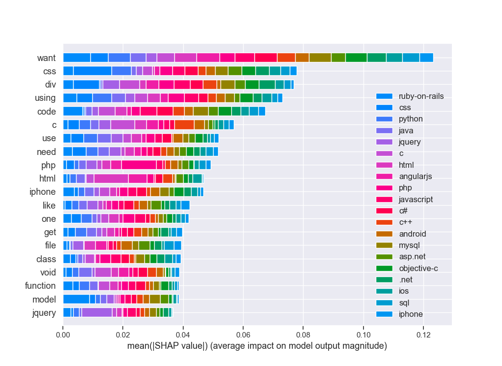
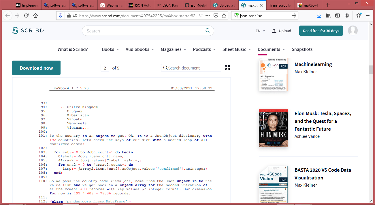
we do have a high accuracy to predict the language from the post question, but the success is based on a self reference in the post, most of the posts do have a hint like :

# post                                                                                    tag

0 how do i move something in rails i m a progr…    ruby-on-rails

39128 my python cgi script for sound hangs when played … … python

the hint is “something in rails” or model that belongs to ruby-on-rails tag!

I checked this with a routine to ask which words of the target class (tags) are in the posts:

sr=[]
>>> for it in set(df.tags):
... al=len(df[df.post.str.contains(it,regex=False)])
... print(it, al)
... sr.append(it+' '+str(al))

[‘.net 3743’, ‘android 1598’, ‘angularjs 1014’, ‘asp.net 1203’, ‘c 39915’, ‘c# 1363’, ‘c++ 1304’, ‘css 2581’, ‘html 5547’, ‘ios 2062’, ‘iphone 1496’, ‘java 4213 ‘, ‘javascript 2281’, ‘jquery 2072’, ‘mysql 2014’, ‘objective-c 556’, ‘php 2513’, ‘python 1565’, ‘ruby-on-rails 23’, ‘sql 4222’]

ruby-on-rails is low with 23 but the hint is ruby in a post:

also “model” is the most important feature to detect a ruby related question in a post!

>>> len(df[df.post.str.contains(‘ruby’,regex=False)])
490

>>> len(df[df.post.str.contains(‘model’,regex=False)])
1692

shap_langimpactFigure_2stopwords2tagsinposts

At least an impact analysis without preprocessing like stopwords, html-cleaning or n-grams settings:

shap_langimpactFigure_2

Even beyond that, it has some very convenient and advanced functions not commonly offered by other libraries:

  • Ensemble Methods: Boosting, Bagging, Random Forest, Model voting and averaging
  • Feature Manipulation: Dimensionality reduction, feature selection, feature analysis
  • Outlier Detection: For detecting outliers and rejecting noise
  • Model selection and validation: Cross-validation, Hyperparamter tuning, and metrics

goldstandard_scikit

maXbox4_25

# Pandas and numpy for data manipulation

# https://github.com/WillKoehrsen/machine-learning-project-walkthrough/blob/master/Machine%Learning%20Project%20Part%203.ipynb

# https://pythondata.com/local-interpretable-model-agnostic-explanations-lime-python/

# https://towardsdatascience.com/explain-nlp-models-with-lime-shap-5c5a9f859b

# Purpose: shows LIME and SHAP together in 3 cases

from __future__ import print_function

import pandas as pd

import numpy as np

# No warnings about setting value on copy of slice

pd.options.mode.chained_assignment = None

pd.set_option(‘display.max_columns’, 60)

# Matplotlib for visualization

import matplotlib.pyplot as plt

#%matplotlib inline

# Set default font size

plt.rcParams[‘font.size’] = 18

from IPython.core.pylabtools import figsize

# Seaborn for visualization

import seaborn as sns

sns.set(font_scale = 2)

# Imputing missing values

from sklearn.preprocessing import Imputer, MinMaxScaler

from sklearn.impute import SimpleImputer

# Machine Learning Models

from sklearn.linear_model import LinearRegression

from sklearn.ensemble import GradientBoostingRegressor

from sklearn import tree

# LIME for explaining predictions

import lime

import lime.lime_tabular

# Read in data into a dataframe

dataf = pd.read_csv(‘data/Energy_and_Water_Data_Disclosure_for_Local_Law_84_2017__Data_for_Calendar_Year_2016_.csv’)

# Display top of dataframe

#print(dataf.head())

# cleaning

# Replace all occurrences of Not Available with numpy not a number

dataf = dataf.replace({‘Not Available’: np.nan})

# Iterate through the columns

for col in list(dataf.columns):

# Select columns that should be numeric

if (‘ft²’ in col or ‘kBtu’ in col or ‘Metric Tons CO2e’ in col or ‘kWh’ in

col or ‘therms’ in col or ‘gal’ in col or ‘Score’ in col):

# Convert the data type to float

dataf[col] = dataf[col].astype(float)

# Histogram of the Raw Energy Star Score

“””

plt.style.use(‘fivethirtyeight’)

plt.hist(dataf[‘ENERGY STAR Score’].dropna(), bins = 100, edgecolor = ‘k’)

plt.xlabel(‘Score’); plt.ylabel(‘Number of Buildings’);

plt.title(‘Energy Star Score Distribution’);

plt.show()

“””

# Create a list of buildings with more than 100 measurements

types = dataf.dropna(subset=[‘ENERGY STAR Score’])

types = types[‘Largest Property Use Type’].value_counts()

types = list(types[types.values > 100].index)

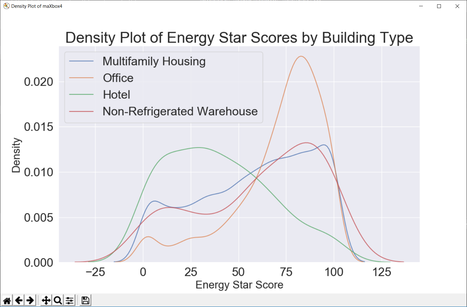
# Plot of distribution of scores for building categories

# A density plot can be thought of as a smoothed histogram because it shows

figsize(12, 10)

#fig = pyplot.gcf()

#figure(‘Density Plot maXbox4’) # 9 is now the title of the window

# Plot each building

for b_type in types:

# Select the building type

subset = dataf[dataf[‘Largest Property Use Type’] == b_type]

# Density plot of Energy Star scores

sns.kdeplot(subset[‘ENERGY STAR Score’].dropna(),

label = b_type, shade = False, alpha = 0.8);

# label the plot

plt.xlabel(‘Energy Star Score’, size = 20); plt.ylabel(‘Density’, size = 20)

plt.title(‘Density Plot of Energy Star Scores by Building Type’, size = 28)

fig = plt.gcf()

fig.canvas.set_window_title(‘Density Plot of maXbox4’)

#fig = plt.figure(‘Density Plot of maXbox4’)

#ig.set_window_title(‘Density Plot maXbox4’)

# Read in data into dataframes

train_features = pd.read_csv(‘data/training_features.csv’)

test_features = pd.read_csv(‘data/testing_features.csv’)

train_labels = pd.read_csv(‘data/training_labels.csv’)

test_labels = pd.read_csv(‘data/testing_labels.csv’)

print(train_features.info())

# print(train_labels.info())

# Create an imputer object with a median filling strategy

#imputer = Imputer(strategy=’median’)

#imputer = SimpleImputer(missing_values = np.nan, strategy = ‘mean’,verbose=0)

imputer = SimpleImputer(strategy = ‘median’,verbose=1)

# Train on the training features

imputer.fit(train_features)

# Transform both training data and testing data

X = imputer.transform(train_features)

X_test = imputer.transform(test_features)

# Sklearn wants the labels as one-dimensional vectors

y = np.array(train_labels).reshape((-1,))

y_test = np.array(test_labels).reshape((-1,))

# print(train_features.info())

# Function to calculate mean absolute error

def mae(y_true, y_pred):

return np.mean(abs(y_true y_pred))

model = GradientBoostingRegressor(loss=‘lad’, max_depth=5, max_features=None,

min_samples_leaf=6, min_samples_split=6,

n_estimators=800, random_state=42)

model.fit(X, y)

# Make predictions on the test set

model_pred = model.predict(X_test)

print(‘Final Model Performance on the test set: MAE = %0.4f’ % mae(y_test, model_pred))

print(‘\n’)

# Find the residuals

residuals = abs(y_test model_pred)

print(residuals)

# Extract the most wrong prediction

wrong = X_test[np.argmax(residuals), :]

# Exact the worst and best prediction

#wrong = X_test_reduced[np.argmax(residuals), :]

right = X_test[np.argmin(residuals), :]

print(‘REs Prediction: %0.4f’ % np.argmax(residuals))

print(‘Actual Value: %0.4f’ % y_test[np.argmax(residuals)])

# Extract the feature importances into a dataframe

feature_results = pd.DataFrame({‘feature’: list(train_features.columns),

‘importance’: model.feature_importances_})

# Show the top 10 most important

feature_results = feature_results.sort_values(‘importance’, ascending = False).reset_index(drop=True)

# Extract the names of the most important features

most_important_features = feature_results[‘feature’][:10]

print(feature_results.head(10))

print(most_important_features)

# pres test

for i in range(10):

try :

x = list(most_important_features[0:])

except IndexError:

print(‘IndexError, list = ‘ + str(most_important_features) + ‘, index = ‘ + str(i))

# train_features is the dataframe of training features

feature_list = list(train_features.columns)

# Create a lime explainer object

explainer = lime.lime_tabular.LimeTabularExplainer(training_data = X_test,

mode = ‘regression’,

training_labels = y, #,

feature_names = feature_list)

# Display the predicted and true value for the wrong instance

print(‘Prediction: %0.4f’ % model.predict(wrong.reshape(1, 1)))

print(‘Actual Value: %0.4f’ % y_test[np.argmax(residuals)])

# Explanation for wrong prediction

wrong_exp = explainer.explain_instance(data_row = wrong,

predict_fn = model.predict)

# Plot the prediction explaination

figsize(16, 6)

wrong_exp.as_pyplot_figure()

plt.title(‘Explanation of Prediction’, size = 28)

plt.xlabel(‘Effect on Prediction’, size = 22)

#plt.show()

# Let’s graph the feature importances to compare visually.

# https://github.com/WillKoehrsen/machine-learning-project-walkthrough/blob/master/Machine%20Learning%20Project%20Part%ipynb

figsize(12, 6)

#plt.style.use(‘fivethirtyeight’)

# Plot the 10 most important features in a horizontal bar chart

feature_results.loc[:9, :].plot(x = ‘feature’, y = ‘importance’,

edgecolor = ‘k’,

kind=‘barh’, color = ‘blue’);

plt.xlabel(‘Relative Importance’, size = 15); plt.ylabel()

plt.title(‘Feature Importances from Random Forest’, size = 20)

plt.show()

# For example, SHAP has a tree explainer that runs fast on trees, such as gradient

# Load Boston Housing Data


import shap

from sklearn.model_selection import train_test_split

import sklearn

import time

X,y = shap.datasets.boston()

X_train,X_test,y_train,y_test = train_test_split(X, y, test_size=0.2, random_state=0)

X,y = shap.datasets.boston()

X_train,X_test,y_train,y_test = train_test_split(X, y, test_size=0.2, random_state=0)

# K Nearest Neighbor

knn = sklearn.neighbors.KNeighborsRegressor()

knn.fit(X_train, y_train)

# Create the SHAP Explainers

# SHAP has the following explainers: deep, gradient, kernel, linear, tree, sampling


# Must use Kernel method on knn

# Summarizing the data with k-Means is a trick to speed up the processing

“””


Rather than use the whole training set to estimate expected values, we summarize with


a set of weighted kmeans, each weighted by the number of points they represent.


Running without kmeans took 1 hr 6 mins 7 sec. 
Running with kmeans took 2 min 47 sec.


Boston Housing is a small dataset.


Running SHAP on models that require the Kernel method becomes prohibitive.


”””

# build the kmeans summary

X_train_summary = shap.kmeans(X_train, 10)

# using the kmeans summary

“””

t0 = time.time()

explainerKNN = shap.KernelExplainer(knn.predict,X_train_summary)

shap_values_KNN_test = explainerKNN.shap_values(X_test)

t1 = time.time()

timeit=t1-t0

timeit

“””

# without kmeans# a test run took 3967.6232330799103 seconds

“””

t0 = time.time()

explainerKNN = shap.KernelExplainer(knn.predict, X_train)

shap_values_KNN_test = explainerKNN.shap_values(X_test)

t1 = time.time()

timeit=t1-t0timeit

“””

# now we can plot the SHAP explainer

j = int

j = 10

#shap.force_plot(explainerKNN.expected_value, shap_values_KNN_test[j], X_test.iloc[[j]])

#Getting started with Local Interpretable Model-agnostic Explanations (LIME)

# https://pythondata.com/local-interpretable-model-agnostic-explanations-lime-python/

from sklearn.datasets import load_boston

boston = load_boston()

print (boston[‘DESCR’])

rf = sklearn.ensemble.RandomForestRegressor(n_estimators=1000)

train, test, labels_train, labels_test = train_test_split(boston.data, boston.target, train_size=0.80)

rf.fit(train, labels_train)

#Now that we have a Random Forest Regressor trained, we can check some of the accuracy measures.

print(‘Random Forest MSError’, np.mean((rf.predict(test) labels_test) ** 2))

# Tbe MSError is: 7.561741634411746 – 10.45. Now, let’s look at the MSError when predicting the mean.

print(‘MSError when predicting the mean’, np.mean((labels_train.mean() labels_test) ** 2))

#To implement LIME, we need to get the categorical features from our data and then build an ‘explainer’.

categorical_features = np.argwhere(

np.array([len(set(boston.data[:,x]))

for x in range(boston.data.shape[1])]) <= 10).flatten()

print(categorical_features)

explainer = lime.lime_tabular.LimeTabularExplainer(train,

feature_names=boston.feature_names,

class_names=[‘price’],

categorical_features=categorical_features,

verbose=True, mode=‘regression’)

#Now, we can grab one of our test values and check out our prediction(s). Here, we’ll grab the 100th test

#value and check the prediction and see what the explainer has to say about it.

#https://shirinsplayground.netlify.com/2018/06/keras_fruits_lime/

i = 100

exp = explainer.explain_instance(test[i], rf.predict, num_features=5)

#print(‘available_labels(): ‘,exp.available_labels())

#raise NotImplementedError(‘Not supported for regression explanations.’)

exp.show_in_notebook(show_table=True)

exp.save_to_file(‘data/limeexplain34.html’)

# Plot the prediction explanation

#exp.as_pyplot_figure();

# plt.show()

# print(exp.as_list(label=8))

print (‘\n’.join(map(str, exp.as_list(label=8))))

# https://towardsdatascience.com/explain-nlp-models-with-lime-shap-5c5a9f84d59b

import pandas as pd

import numpy as np

import sklearn

import sklearn.ensemble

import sklearn.metrics

from sklearn.utils import shuffle

from io import StringIO

import re

from bs4 import BeautifulSoup

from nltk.corpus import stopwords

from sklearn.model_selection import train_test_split

from sklearn.feature_extraction.text import CountVectorizer

from sklearn.linear_model import LogisticRegression

from sklearn.metrics import accuracy_score, f1_score, precision_score, recall_score

import lime

from lime import lime_text

from lime.lime_text import LimeTextExplainer

from sklearn.pipeline import make_pipeline

df = pd.read_csv(‘data/stack-overflow-data.csv’)

df = df[pd.notnull(df[‘tags’])]

#print (df.groupby(‘tags’).count().sort_values([‘tags’]))

df = df.sample(frac=0.5, random_state=99).reset_index(drop=True)

df = shuffle(df, random_state=22)

df = df.reset_index(drop=True)

df[‘class_label’] = df[‘tags’].factorize()[0]

class_label_df = df[[‘tags’, ‘class_label’]].drop_duplicates().sort_values(‘class_label’)

label_to_id = dict(class_label_df.values)

id_to_label = dict(class_label_df[[‘class_label’, ‘tags’]].values)

print(df.info())

print(df.head(5))

REPLACE_BY_SPACE_RE = re.compile(r'[/(){}\[\]\|@,;]’)

BAD_SYMBOLS_RE = re.compile(‘[^0-9a-z #+_]’)

# STOPWORDS = set(stopwords.words(‘english’))

def clean_text(text):

“””

text: a string

return: modified initial string

“””

text = BeautifulSoup(text, “lxml”).text

# HTML decoding. BeautifulSoup’s text attribute will return a string stripped of any HTML tags and metadata.

text = text.lower() # lowercase text

text = REPLACE_BY_SPACE_RE.sub(‘ ‘, text)

# replace REPLACE_BY_SPACE_RE symbols by space in text. substitute the matched string in REPLACE_BY_SPACE_RE with space.

text = BAD_SYMBOLS_RE.sub(, text)

# remove symbols which are in BAD_SYMBOLS_RE from text. substitute the matched string in BAD_SYMBOLS_RE

# with nothing.

# text = ‘ ‘.join(word for word in text.split() if word not in STOPWORDS) # remove stopwors from text

return text

df[‘post’] = df[‘post’].apply(clean_text)

list_corpus = df[“post”].tolist()

list_labels = df[“class_label”].tolist()

print(set(df[‘tags’]))

print (df.groupby(‘tags’).count())

X_train, X_test, y_train, y_test = train_test_split(list_corpus, list_labels, test_size=0.2, random_state=40)

vectorizer = CountVectorizer(analyzer=‘word’, token_pattern=r’\w{1,}’,

ngram_range=(1, 3), stop_words = ‘english’, binary=True)

train_vectors = vectorizer.fit_transform(X_train)

test_vectors = vectorizer.transform(X_test)

logreg = LogisticRegression(n_jobs=1, C=1e5)

logreg.fit(train_vectors, y_train)

pred = logreg.predict(test_vectors)

accuracy = accuracy_score(y_test, pred)

precision = precision_score(y_test, pred, average=‘weighted’)

recall = recall_score(y_test, pred, average=‘weighted’)

f1 = f1_score(y_test, pred, average=‘weighted’)

print(“accuracy = %.3f, precision = %.3f, recall = %.3f, f1 = %.3f” % (accuracy, precision, recall, f1))

c = make_pipeline(vectorizer, logreg)

class_names=list(df.tags.unique())

explainer = LimeTextExplainer(class_names=class_names)

idx = 1877

exp = explainer.explain_instance(X_test[idx], c.predict_proba, num_features=6, labels=[4, 8])

print(‘Document id: %d’ % idx)

print(‘Predicted class =’, class_names[logreg.predict(test_vectors[idx]).reshape(1,-1)[0,0]])

print(‘True class: %s’ % class_names[y_test[idx]])

# We randomly select a document in test set, it happens to be a document that labeled as sql,

# and our model predicts it as sql as well. Using this document, we generate explanations

# for label 4 which is sql and label 8 which is python.

print (‘Explanation for class %s’ % class_names[4])

print (‘\n’.join(map(str, exp.as_list(label=4))))

print (‘Explanation for class %s’ % class_names[8])

print (‘\n’.join(map(str, exp.as_list(label=8))))

# We are going to generate labels for the top 2 classes for this document.

exp = explainer.explain_instance(X_test[idx], c.predict_proba, num_features=6, top_labels=2)

print(exp.available_labels())

exp.show_in_notebook(text=y_test[idx], labels=(4,))

exp.save_to_file(‘data/stackoverflowlimeexplain34_sql.html’)

exp.show_in_notebook(text=y_test[idx], labels=(8,))

exp.save_to_file(‘data/stackoverflowlimeexplain38_python.html’)

#exp = explainer.explain_instance(X_test[idx], c.predict_proba, num_features=6, top_labels=2)

#print(exp.available_labels())

#exp.show_in_notebook(text=False)

#exp.as_pyplot_figure(labels = exp.available_labels());

#plt.show()

# It gives us sql and python.

# Interpreting text predictions with SHAP

# https://towardsdatascience.com/explain-nlp-models-with-lime-shap-5c5a9f84d59b

from sklearn.preprocessing import MultiLabelBinarizer

import tensorflow as tf

from tensorflow.keras.preprocessing import text

import keras.backend.tensorflow_backend as K

K.set_session

import shap

tags_split = [tags.split(‘,’) for tags in df[‘tags’].values]

tag_encoder = MultiLabelBinarizer()

tags_encoded = tag_encoder.fit_transform(tags_split)

num_tags = len(tags_encoded[0])

train_size = int(len(df) * .8)

print(‘lang labels count: ‘,num_tags)

y_train = tags_encoded[: train_size]

y_test = tags_encoded[train_size:]

class TextPreprocessor(object):

def __init__(self, vocab_size):

self._vocab_size = vocab_size

self._tokenizer = None

def create_tokenizer(self, text_list):

tokenizer = text.Tokenizer(num_words = self._vocab_size)

tokenizer.fit_on_texts(text_list)

self._tokenizer = tokenizer

def transform_text(self, text_list):

text_matrix = self._tokenizer.texts_to_matrix(text_list)

return text_matrix

VOCAB_SIZE = 500

train_post = df[‘post’].values[: train_size]

test_post = df[‘post’].values[train_size: ]

processor = TextPreprocessor(VOCAB_SIZE)

processor.create_tokenizer(train_post)

X_train = processor.transform_text(train_post)

X_test = processor.transform_text(test_post)

def create_model(vocab_size, num_tags):

model = tf.keras.models.Sequential()

model.add(tf.keras.layers.Dense(50, input_shape = (VOCAB_SIZE,), activation=‘relu’))

model.add(tf.keras.layers.Dense(25, activation=‘relu’))

model.add(tf.keras.layers.Dense(num_tags, activation=‘sigmoid’))

model.compile(loss = ‘binary_crossentropy’, optimizer=‘adam’, metrics = [‘accuracy’])

return model

model = create_model(VOCAB_SIZE, num_tags)

model.fit(X_train, y_train, epochs = 2, batch_size=128, validation_split=0.1)

print(‘Eval loss/accuracy:{}’.format(model.evaluate(X_test, y_test, batch_size = 128)))

attrib_data = X_train[:200]

explainer = shap.DeepExplainer(model, attrib_data)

num_explanations = 20

shap_vals = explainer.shap_values(X_test[:num_explanations])

words = processor._tokenizer.word_index

word_lookup = list()

for i in words.keys():

word_lookup.append(i)

word_lookup = [] + word_lookup

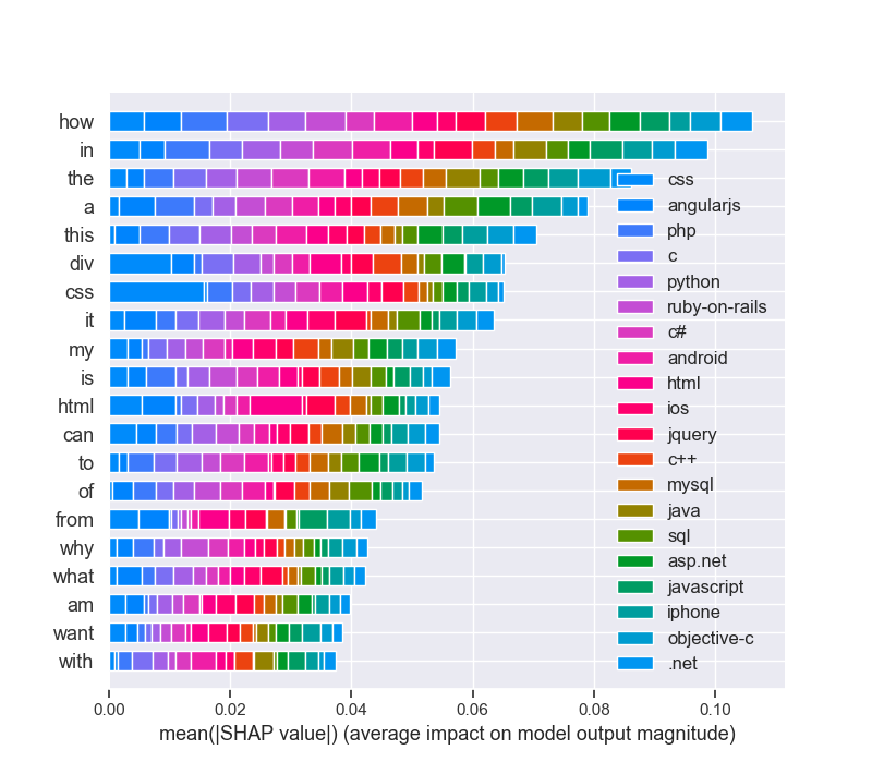
shap.summary_plot(shap_vals, feature_names=word_lookup, class_names=tag_encoder.classes_)

print(‘end of EAI LIME & SHAP box trix___KERAS____’)

“””

ERROR: sonnet 0.1.6 has requirement networkx==1.8.1, but you’ll have networkx 2.4 which is incompatible.

Installing collected packages: progressbar, lime, networkx

Found existing installation: networkx 1.8.1

Uninstalling networkx-1.8.1:

Successfully uninstalled networkx-1.8.1

Successfully installed lime-0.1.1.37 networkx-2.4 progressbar-2.5

PS r C:\maXbox\maxbox3\maxbox3\maXbox3\crypt\viper2> pip3 install shap

Collecting shap

Downloading r https://files.pythonhosted.org/packages/c0/e4/8cb0cbe60af287d66abff92d5c10ec2a1a501b2ac68779bd008a3b473d3b/shap-0.34.0-cp37-cp37m-win_amd64.whl

(298kB)

|████████████████████████████████| 307kB 1.7MB/s

Requirement already satisfied: numpy in \lib\site-packages (from shap) (1.16.3)

Requirement already satisfied: scikit-learn in \lib\site-packages (from shap) (0.20.3)

Requirement already satisfied: pandas in lib\site-packages (from shap) (0.24.2)

Requirement already satisfied: scipy in \lib\site-packages (from shap) (1.2.0)

Requirement already satisfied: tqdm>4.25.0 in \lib\site-packages (from shap) (4.31.1)

Requirement already satisfied: pytz>=2011k in \python37\lib\site-packages (from pandas->shap) (2019.1)

Requirement already satisfied: python-dateutil>=2.5.0 in python37\lib\site-packages (from pandas->shap) (2.7.5)

Requirement already satisfied: six>=1.5 in \python37\lib\site-packages (from python-dateutil>=2.5.0->pandas->shap) (1.12.0)

Installing collected packages: shap

Successfully installed shap-0.34.0

WARNING: You are using pip version 19.1, however version 20.0.1 is available.

You should consider upgrading via the ‘python -m pip install –upgrade pip’ command.

PS C:\maXbox\maxbox3\maxbox3\maXbox3\crypt\viper2>

In the first two parts of this project, we implemented the first 6 steps of the machine learning pipeline:

Data cleaning and formatting

Exploratory data analysis

Feature engineering and selection

Compare several machine learning models on a performance metric

Perform hyperparameter tuning on the best model to optimize it for the problem

Evaluate the best model on the testing set

Interpret the model results to the extent possible

Draw conclusions and write a well-documented report

Here’s how to interpret the plot: Each entry on the y-axis indicates one value of a variable and the red and green bars show

the effect this value has on the prediction. For example, the top entry says the Site EUI is greater than 95.90 which subtracts

about 40 points from the prediction. The second entry says the Weather Normalized Site Electricity Intensity is less

than 3.80 which adds about 10 points to the prediction. The final prediction is an intercept term plus the sum of each

of these individual contributions.

library(keras) # for working with neural nets

library(lime) # for explaining models

library(magick) # for preprocessing images

library(ggplot2) # for additional plotting

Intercept 26.62833899477304

Prediction_local [16.78374133]

Right: 8.788700000000027

<IPython.core.display.HTML object>

(‘LSTAT > 17.09’, -4.89649843884296)

(‘5.91 < RM <= 6.23’, -3.913881918724065)

(‘NOX > 0.62’, -1.1532969589236963)

(‘DIS <= 2.11’, 0.8798771793667672)

(‘18.95 < PTRATIO <= 20.20’, -0.76079752709186)

end of EAI box trix___

Intercept 23.888469758845538

Prediction_local [24.06097282]

Right: 25.466100000000058

<IPython.core.display.HTML object>

(‘6.21 < RM <= 6.60’, -2.398134087581002)

(‘7.20 < LSTAT <= 11.30’, 1.914742343880133)

(‘TAX <= 281.00’, 0.7204900819903772)

(‘CHAS=0’, -0.5690170981066284)

(‘17.38 < PTRATIO <= 19.05’, 0.5044218222752127)

def explain_instance(data_row, predict_fn, labels=(1,), top_labels=None, num_features=10,

num_samples=5000, distance_metric=’euclidean’, model_regressor=None)

Generates explanations for a prediction.

First, we generate neighborhood data by randomly perturbing features from the instance (see __data_inverse).

We then learn locally weighted linear models on this neighborhood data to explain each of the classes in an

interpretable way (see lime_base.py).

Args:

data_row: 1d numpy array or scipy.sparse matrix, corresponding to a row

predict_fn: prediction function. For classifiers, this should be a

function that takes a numpy array and outputs prediction

probabilities. For regressors, this takes a numpy array and

returns the predictions. For ScikitClassifiers, this is

`classifier.predict_proba()`. For ScikitRegressors, this

is `regressor.predict()`. The prediction function needs to work

on multiple feature vectors (the vectors randomly perturbed

from the data_row).

labels: iterable with labels to be explained.

top_labels: if not None, ignore labels and produce explanations for

the K labels with highest prediction probabilities, where K is

this parameter.

num_features: maximum number of features present in explanation

num_samples: size of the neighborhood to learn the linear model

distance_metric: the distance metric to use for weights.

model_regressor: sklearn regressor to use in explanation. Defaults

to Ridge regression in LimeBase. Must have model_regressor.coef_

and ‘sample_weight’ as a parameter to model_regressor.fit()

Returns:

An Explanation object (see explanation.py) with the corresponding

explanations.

Q: Each time I run the demo I got different explanation!! RAD=24 is not always the most positive

A: That’s not a surprise.

LIME is ‘an algorithm that can explain the predictions of any classifier or regressor in a faithful way,

by approximating it locally with an interpretable model’

I would expect it to provide slightly different results when you run it with this dataset.

“””

strommarktjune2020

20170415_train_fhafen


Its 3 hour AM with the negative Peak on 4.12. and strong wind gale (almost stormy weather)
Design a site like this with WordPress.com
Get started