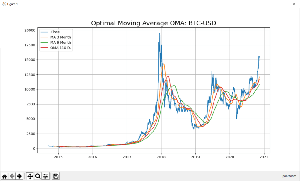
In this blog of python for stock market, we will discuss two ways to predict stock with Python- Support Vector Regression (SVR) with Optimal Moving Average (OMA).

A time-series is a series of data points indexed in time order and it is used to predict the future based on the previous observed values. Time series are very frequently plotted via line charts. Time series are used in statistics , weather forecasting, stock price prediction, pattern recognition, earthquake prediction, e.t.c.
Program PythonShell3_SVR_21_Integrate;

//# -*- coding: utf-8 -*-  http://127.0.0.1:8080
//import scrapy - precondition note: change pyscript path of 991_oma_chartregression2.py

Const
 PYPATH='C:\Users\max\AppData\Local\Programs\Python\Python36-32\';
 PYPATH64='C:\Users\max\AppData\Local\Programs\Python\Python36\';

 PYCODE='C:\Users\max\SkyDrive\IBZ_Prozesstechnik_2016\hellomaxbox\.vscode\urlschemaload.py';
 PYSCRIPT= 'C:\maXbox\mX46210\DataScience\confusionlist\991_oma_chartregression2.py';

 PYFILE = 'input("prompt: ")'+CRLF+
          'def mygauss3():  '+CRLF+
          '#    i=0         '+CRLF+
          '     return sum(i for i in range(101))'+CRLF+
          '#    i=sum(i for i in range(101))'+CRLF+
          '#    print(i)   '+CRLF+
          '                '+CRLF+
          'print(mygauss3())'+CRLF+
          'k=input("press close to exit") '+CRLF+
          '#input("prompt: ")';

 PYFILE1    =//                "source": [
                'listOfNumbers = [1, 2, 3, 4, 5, 6]'+CRLF+
                                   ''+CRLF+
                                   'for number in listOfNumbers:'+CRLF+
                                   '    print(number)'+CRLF+
                                   '    if (number % 2 == 0):'+CRLF+
                                   '        print(''\"is even\"'')'+CRLF+
                                   '    else:'+CRLF+
                                   '        print(''\"is odd\"'')'+CRLF+
                                   '        '+CRLF+
                                   '    print (''\"All done.\"'')'+CRLF;

 PYFILE2 = ' def'+CRLF;

 PYFILE3 = 'sum(i for i in range(101))';

 PYFILE4 = 'def mygauss3():  '+CRLF+
          '#    i=0         '+CRLF+
          '     return sum(i for i in range(101))'+CRLF+
          '#    i=sum(i for i in range(101))'+CRLF+
          '#    print(i)   '+CRLF+
          '                '+CRLF+
          'print(mygauss3())'+CRLF+
          '';

PYSCRIPT5 =
'import numpy as np'+CRLF+
'import matplotlib.pyplot as plt'+CRLF+
'import sys'+CRLF+
'#from sklearn import tree'+CRLF+
'from sklearn.svm import SVC'+CRLF+
'#from sklearn.ensemble import RandomForestClassifier'+CRLF+
'#from sklearn.linear_model import LogisticRegression'+CRLF+
'from sklearn.preprocessing import StandardScaler'+CRLF+
'from sklearn.metrics import accuracy_score'+CRLF+
'from sklearn.model_selection import train_test_split'+CRLF+
' '+CRLF+
' '+CRLF+
'# Quotes from Yahoo finance and find optimal moving average'+CRLF+
'import pandas_datareader.data as web'+CRLF+
'  '+CRLF+
'#DataMax - Predict for 30 days; Predicted has data of Adj. Close shifted up by 30 rows'+CRLF+
'forecast_len=80  #default oma is 5'+CRLF+
'YQUOTES = "^SSMI"'+CRLF+
'PLOT = "Y"'+CRLF+
'try:'+CRLF+
'  forecast_len = int(sys.argv[1])'+CRLF+
'  #forecast_len= int(" ".join(sys.argv[1:]))'+CRLF+
'  YQUOTES = str(sys.argv[2])'+CRLF+
'  PLOT = str(sys.argv[3])'+CRLF+
'except:'+CRLF+
'  forecast_len= forecast_len'+CRLF+
'  YQUOTES = YQUOTES'+CRLF+
'  '+CRLF+
'#YQUOTES = "BTC-USD"  #^GDAXI" , "^SSMI" , "^GSPC" (S&P 500 ) - ticker="GOOGL"'+CRLF+
'try: '+CRLF+
'  df= web.DataReader(YQUOTES, data_source="yahoo",start="09-11-2010")'+CRLF+
'except:'+CRLF+
'  YQUOTES = "^SSMI"'+CRLF+
'  df= web.DataReader(YQUOTES, data_source="yahoo",start="09-11-2010")'+CRLF+
'  print("Invalid Quote Symbol got ^SSMI instead")'+CRLF+
'  '+CRLF+
'#data = " ".join(sys.argv[1:])'+CRLF+
'print ("get forecast len:",forecast_len, "for ", YQUOTES)'+CRLF+
'quotes = df'+CRLF+
'print(quotes.info(5))'+CRLF+
'print(quotes["Close"][:5])'+CRLF+
'print(quotes["Close"][-3:])'+CRLF+
'df["_SMI_20"] = df.iloc[:,3].rolling(window=20).mean()'+CRLF+
'df["_SMI_60"] = df.iloc[:,3].rolling(window=60).mean()'+CRLF+
'df["_SMI_180"] = df.iloc[:,3].rolling(window=180).mean()'+CRLF+
'df["_SMI_OMA"] = df.iloc[:,3].rolling(window=forecast_len).mean()'+CRLF+
'  '+CRLF+
'#"""'+CRLF+
'if PLOT=="Y":'+CRLF+
'   x_ax_time = quotes.index #range(len(df))'+CRLF+
'   plt.figure(figsize=[12,7])'+CRLF+
'   plt.grid(True)'+CRLF+
'   plt.title("Optimal Moving Average OMA: "+YQUOTES, fontsize=18)'+CRLF+
'   plt.plot(x_ax_time, quotes["Close"], label="Close")'+CRLF+
'   plt.plot(x_ax_time, df["_SMI_60"],label="MA 3 Month")'+CRLF+
'   plt.plot(x_ax_time, df["_SMI_180"],label="MA 9 Month")'+CRLF+
'   plt.plot(x_ax_time, df["_SMI_OMA"],label= "OMA "+str(forecast_len)+" D.")'+CRLF+
'   #plt.xlabel("days", fontsize=15)'+CRLF+
'   # plt.plot_date(quotes.index, quotes["Close"])'+CRLF+
'   plt.legend(loc=2)'+CRLF+
'   plt.show()'+CRLF+
'#"""'+CRLF+
'  '+CRLF+
'dates = quotes.index'+CRLF+
'dates = dates[1:]'+CRLF+
'#closing_values = np.array([quote[3] for quote in quotes])'+CRLF+
'#volume_of_shares = np.array([quote[5] for quote in quotes])[1:]'+CRLF+
'closing_values = np.array(quotes["Close"])'+CRLF+
'volume_of_shares = np.array(quotes["Volume"])'+CRLF+
'  '+CRLF+
'#Predict for 30 days; Predicted has Quotes of Close shifted up by 30 rows'+CRLF+
'ytarget= quotes["Close"].shift(-forecast_len)'+CRLF+
'ytarget= ytarget[:-forecast_len]'+CRLF+
'Xdata= closing_values[:-forecast_len]'+CRLF+
'#print("Offset shift:",ytarget[:10])'+CRLF+
'  '+CRLF+
'# Feature Scaling'+CRLF+
'#sc_X = StandardScaler()'+CRLF+
'#sc_y = StandardScaler()'+CRLF+
'#Xdata = sc_X.fit_transform(Xdata.reshape(-1,1))'+CRLF+
'#You need to do this is that pandas Series objects are by design one dimensional.'+CRLF+
'#ytarget = sc_y.fit_transform(ytarget.values.reshape(-1,1))'+CRLF+
'   '+CRLF+
'from sklearn.svm import SVR'+CRLF+
'# Split datasets into training and test sets (80% and 20%)'+CRLF+
'print("target shape len2: ",len(ytarget),len(Xdata))'+CRLF+
'x_train,x_test,y_train,y_test=train_test_split(Xdata,ytarget,test_size=0.2, \'+CRLF+
'                                                       random_state= 72)'+CRLF+
'print("xtrain shape len3: ",len(x_train),len(y_train))'+CRLF+
'   '+CRLF+
'# - Create SVR model and train it'+CRLF+
'svr_rbf= SVR(kernel="rbf",C=1e3,gamma=0.1)'+CRLF+
'x_train = x_train.reshape(-1,1)'+CRLF+
'svr_rbf.fit(x_train,y_train)'+CRLF+
'   '+CRLF+
'# Predicting single value as new result'+CRLF+
'print("predict old in :", forecast_len, svr_rbf.predict([quotes["Close"][:1]]))'+CRLF+
'print("prepredict now in :", forecast_len, svr_rbf.predict([quotes["Close"][-1:]]))'+CRLF+
'    '+CRLF+
'#DBASTAr - Get score'+CRLF+
'svr_rbf_confidence=svr_rbf.score(x_test.reshape(-1,1),y_test)'+CRLF+
'print(f"SVR Confidence: {round(svr_rbf_confidence*100,2)}%")';

 ACTIVESCRIPT = PYSCRIPT5;

 function CompareFilename(List: TStringList; Index1, Index2: Integer): Integer;
var
  fn1, fn2: String;
begin
  fn1 := List.Names[Index1];
  fn2 := List.Names[Index2];
  Result := CompareString(fn1, fn2);
end;

function CompareFileSize(List: TStringList; Index1, Index2: Integer): Integer;
var
  sz1, sz2: Int64;
begin
  sz1 := StrToInt(List.ValueFromIndex[Index1]);
  sz2 := StrToInt(List.ValueFromIndex[Index2]);
  Result := ord(CompareValueI(sz1, sz2));
end;

Function GetValueFromIndex(R: TStringList; Index: Integer):String;
var
  S: string;
  i: Integer;
begin
  S := R.Strings[Index];
  i := Pos('=', S);
  if I > 0 then
    result := Copy(S, i+1, MaxInt)
  else
    result := '';
end;

Function dummy(Reqlist: TStringList):String;
var
  i: Integer;
  RESULTv: string;
begin
  for i := 0 to ReqList.Count-1 do
    RESULTv := RESULTv + Reqlist.Names[i] + ' -> ' + GetValueFromIndex(Reqlist, i);
  result := RESULTv;
end;

 var fcast: integer;
     olist: TStringlist;
     dosout, theMaxOMA, QuoteSymbol: string;
     Yvalfloat: array[1..500] of double; //TDynfloatArray;
     //theMaxFloat: double;

     RUNSCRIPT: string;

begin //@main

  //saveString(exepath+'mygauss.py',ACTIVESCRIPT);
  saveString(exepath+'991_oma_chartregression5.py',ACTIVESCRIPT);
  sleep(300)
  //if fileExists(PYPATH+'python.exe') then
   //if fileExists(PYSCRIPT) then begin
   if fileExists(exepath+'991_oma_chartregression5.py') then begin
      RUNSCRIPT:= exepath+'991_oma_chartregression5.py';
     //ShellExecute3('cmd','/k '+PYPATH+'python.exe && '+PYFILE +'&& mygauss3()'
     //                                  ,secmdopen);
      { ShellExecute3('cmd','/k '+PYPATH+
                        'python.exe && exec(open('+exepath+'mygauss.py'').read())'
                        ,secmdopen);
                 }
     { ShellExecute3('cmd','/k '+PYPATH+
                        'python.exe '+exepath+'mygauss.py', secmdopen); }
     // ShellExecute3(PYPATH+'python.exe ',exepath+'mygauss.py'
     //                   ,secmdopen);
     maxform1.console1click(self);
     memo2.height:= 205;
     // maxform1.shellstyle1click(self);
     // writeln(GetDosOutput(PYPATH+'python.exe '+PYSCRIPT,'C:\'));
    fcast:= 120;      //first forecast with plot
    QuoteSymbol:= 'BTC-USD'; //'BTC-USD'; //^SSMI    TSLA
    olist:= TStringlist.create;
    olist.NameValueSeparator:= '=';
    //olist.Sorted:= True;
    //olist.CustomSort(@CompareFileName)
    //GetDosOutput('py '+PYSCRIPT+' '+itoa(fcast)+' '+QuoteSymbol+' "Y"','C:\');
    GetDosOutput('py '+RUNSCRIPT+' '+itoa(fcast)+' '+QuoteSymbol+' "Y"','C:\');

    for it:= 20 to 130 do
       if it mod 5=0 then begin
         //(GetDosOutput('py '+PYSCRIPT+' '+itoa(it)+' "BTC-USD"'+ 'Plot?','C:\'));
         dosout:= GetDosOutput('py '+RUNSCRIPT+' '+itoa(it)+' '+QuoteSymbol+' "N"','C:\');
         writeln(dosout)
         with TRegExpr.Create do begin
            //Expression:=('SVR Confidence: ([0-9\.%]+).*');
            Expression:=('SVR Confidence: ([0-9\.]+).*');
            if Exec(dosout) then begin
              PrintF('Serie %d  : %s',[it, Match[1]]);
              olist.add(Match[1]+'='+itoa(it));
              Yvalfloat[it]:= strtofloat(Copy(match[1],1,5));
              //MaxFloatArray
            end;
          Free;
         end;
       end;
     writeln(CR+LF+olist.text)
     writeln('OMA from key value list2: '+floattostr(MaxFloatArray(Yvalfloat)))
     TheMaxOMA:= olist.Values[floattostr(MaxFloatArray(Yvalfloat))];
     writeln('OMA for Chart Signal: '+TheMaxOMA);
     olist.Free;
    (GetDosOutput('py '+RUNSCRIPT+' '+(TheMaxOMA)+' '+QuoteSymbol+' "Y"','C:\'));
   end;
End.

ref: https://docs.scrapy.org/en/latest/topics/link-extractors.html

https://doc.scrapy.org/en/latest/topics/architecture.html

https://www.rosettacode.org/wiki/Cumulative_standard_deviation#Pascal

https://www.kaggle.com/vsmolyakov/keras-cnn-with-fasttext-embeddings

https://www.angio.net/pi/bigpi.cgi

This function changes all data into a value between 0 and 1. This is as
 many stocks have skyrocketed or nosedived. Without normalizing, the
 neural network would learn from datapoints with higher values. This could
 create a blind spot and therefore affect predictions. The normalizing is
 done as so:

value = (value - minimum) / maximum

if Exec(memo2.text) then
         for i:=0 to SubExprMatchCount do
            PrintF('Group %d  : %s', [i, Match[i]]);


class ExampleSpider(scrapy.Spider):
    name = 'example'
    #allowed_domains = ['www.ibm.ch']
    allowed_domains = ['127.0.0.1']

    #start_urls = ['http://www.ibm.ch/']
    start_urls = ['http://127.0.0.1:8080']

    def parse(self, response):
        pass


        "source": [
    "import numpy as np\n",
    "\n",
    "A = np.random.normal(25.0, 5.0, 10)\n",
    "print (A)"
   ]
  {
   "cell_type": "markdown",
   "metadata": {
    "deletable": true,
    "editable": true
   },
   "source": [
    "## Activity"
   ]
  },
  {
   "cell_type": "markdown",
   "metadata": {
    "deletable": true,
    "editable": true
   },
   "source": [
    "Write some code that creates a list of integers, loops through each
element of the list, and only prints out even numbers!"
   ]
  },
  {
   "cell_type": "code",
   "execution_count": null,
   "metadata": {
    "collapsed": false,
    "deletable": true,
    "editable": true
   },
   "outputs": [],
   "source": []
  }
 ],
 "metadata": {
  "kernelspec": {
   "display_name": "Python 3",
   "language": "python",
   "name": "python3"
  },
  "language_info": {
   "codemirror_mode": {
    "name": "ipython",
    "version": 3
   },
   "file_extension": ".py",
   "mimetype": "text/x-python",
   "name": "python",
   "nbconvert_exporter": "python",
   "pygments_lexer": "ipython3",
   "version": "3.5.2"
  }
 },
 "nbformat": 4,
 "nbformat_minor": 0
}


// demo of graphviz integration of a C# wrapper for the GraphViz graph generator for dotnet core.
// by Max Kleiner for BASTA
// https://www.nuget.org/packages/GraphViz.NET/
// https://sourceforge.net/projects/maxbox/upload/Examples/EKON/BASTA2020/visout/
// dotnet run C:\maXbox\BASTA2020\visout\BASTA_GraphVizCoreProgram.cs
// dotnet run C:\maXbox\BASTA2020\visout\visout.csproj

using System;
using System.Collections;
using System.Runtime.InteropServices;

using GraphVizWrapper;
using GraphVizWrapper.Commands;
using GraphVizWrapper.Queries;

using Graphviz4Net.Graphs;
//# using ImageFormat.Png;
using System.Drawing.Imaging;
using System.Drawing;
using System.Drawing.Drawing2D;
using System.IO; //memory stream
using System.Diagnostics;


namespace visout

{
    class ProgramGraph
    {

        static void Main(string[] args)
        {
        // These three instances can be injected via the IGetStartProcessQuery,
        //                                               IGetProcessStartInfoQuery and
        //                                               IRegisterLayoutPluginCommand interfaces

        var getStartProcessQuery = new GetStartProcessQuery();
        var getProcessStartInfoQuery = new GetProcessStartInfoQuery();
        var registerLayoutPluginCommand = new RegisterLayoutPluginCommand(getProcessStartInfoQuery, getStartProcessQuery);

        // GraphGeneration can be injected via the IGraphGeneration interface

        var wrapper = new GraphGeneration(getStartProcessQuery,
								               getProcessStartInfoQuery,  registerLayoutPluginCommand);

        //byte[] bitmap = wrapper.GenerateGraph("digraph{a -> b; b -> c; c -> a;}", Enums.GraphReturnType.Png);
        //byte[] bitmap = wrapper.GenerateGraph("digraph{a -> b; b -> d; b -> c; d ->a; a->d;}",
          //                                                        Enums.GraphReturnType.Png);
        byte[] bitmap = wrapper.GenerateGraph("digraph M {R -> A; A -> S; S -> T; T -> A;"
                                                 +"A -> 20 -> 20 [color=green];}",
                                                                  Enums.GraphReturnType.Png);


        using(Image image = Image.FromStream(new MemoryStream(bitmap)))

        {
          image.Save("graphvizoutput3114.png",ImageFormat.Png); // Or Jpg
        }

        //Process.Start(@"graphvizoutput3114.png");
        Process pim = new Process();
        pim.StartInfo = new ProcessStartInfo()
        {
            //CreateNoWindow = true, no mspaint platform!
            Verb = "show",
            FileName = "mspaint.exe", //put the path to the software e.g.
            Arguments=@"C:\maXbox\BASTA2020\visout\graphvizoutput3114.png"
        };
        pim.Start();

            Console.WriteLine("Hello maXbox Core Viz maXbox474 World!");
            Console.WriteLine("Welcome to GraphViz GraphViz.NET 1.0.1");
            unsafe
            {
              GViz gviz = new GViz();
              GViz* p = &gviz;
              //ptr to member operator struct
              DateTime currentDateTime = DateTime.Now;

              p->x = currentDateTime.Year;
              Console.WriteLine(gviz.x);
            }
        }
    }
    struct GViz
    {
        public int x;
    }
}

// https://www.nuget.org/packages/GraphViz.NET/

//https://www.nuget.org/packages/GraphViz4Net/

// https://github.com/helgeu/GraphViz-C-Sharp-Wrapper
// https://github.com/JamieDixon/GraphViz-C-Sharp-Wrapper

// http://fssnip.net/7Rf/title/Generating-GraphViz-images-using-C-wrapper
//https://graphviz.org/gallery/
//https://renenyffenegger.ch/notes/tools/Graphviz/examples/index

//https://www.hanselman.com/blog/AnnouncingNETJupyterNotebooks.aspx
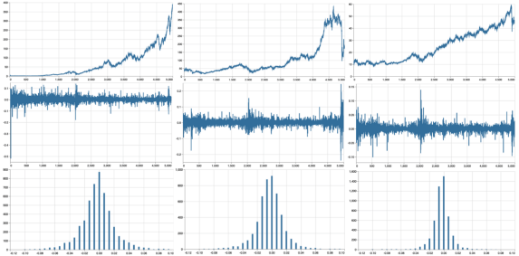
We can see that in the real world, the tails extend further out and a “quiet” day is much more common than in a simple Geometric Brownian Motion, implying the distribution has a higher kurtosis than the normal distribution.
Autocorrelation refers to the degree of correlation of the same variables between two successive time intervals. It measures how the lagged version of the value of a variable is related to the original version of it in a time series.


Tutorials
Description:
Tutorial 00 Function-Coding (Blix the Programmer)
– You’ve always wanted to learn how to build software
Tutorial 01 Procedural-Coding
– All you need to know is that in this program, we have a procedure and a function
Tutorial 02 OO-Programming
– This lesson will introduce you to objects, classes and events.
Tutorial 03 Modular Coding
– Modular programming is subdividing your program into separate subprograms and function blocks or building blocks
Tutorial 04 UML Use Case Coding
– UML is said to address the modelling of manual, as well as parts of systems.
Tutorial 05 Internet Coding
– This lesson will introduce you to Indy Sockets and the library.
Tutorial 06 Network Coding
– This lesson will introduce you to FTP and HTTP.

Tutorial 07 Game Graphics Coding
– This lesson will introduce a simple game called Arcade like Pong.
Tutorial 08 Operating System Coding
– Lesson will introduce various short functions interacting with the OS API.
Tutorial 09 Database Coding
– Introduction to SQL (Structured Query Language) and database connection.
Tutorial 10 Statistic Coding
– We spend time in programming Statistics and in our case with probability.

Tutorial 10 Probability Coding
– Probability theory is required to describe nature and life.


Tutorial 11 Forms Coding
– TApplication, TScreen, and TForm are the classes that form.
Tutorial 12 SQL DB Coding
– SQL Programming V2 with table and db grid.
Tutorial 13 Crypto Coding
– CryptoBox is based on LockBox 3 which is a library for cryptography.
Tutorial 14 Parallel Coding
– I’ll explain you what “blocking” and “non-blocking” calls are.
Tutorial 15 Serial RS232 Coding
– Serial communication is based on a protocol and the standard RS 232.

Tutorial 16 Event Driven Coding
– Event driven programming are usually message based languages
Tutorial 17 Web Server Coding
– This lesson will introduce you to Indy Sockets with the TCP-Server.
Tutorial 18 Arduino System Coding
– Arduino hardware is programmed using a Wiring-based language.
Tutorial 18_3 Arduino RGB LED Coding
– We code a RGB LED light on the Arduino board and breadboard.
- Tutor 18_3 Arduino RGB LED Breadboard and Source LED Zip
Tutorial 18_5 Arduino RGB LED WebSocket
– Web server and their COM interface protocols too.
Tutorial 19 WinCOM /Arduino Coding
– Illustrates what the WinCOM (Component Object Model) interface.
- Tutor 19 WinCOM /Arduino Coding and Source LED COM
Tutorial 20 Regular Expressions RegEx
– A regular expression (RegEx): describes a search pattern of text.

Tutorial 21 Android SONAR: End of 2015
– SonarQube Technical Architecture
- Tutor 21 Android SONAR: 2015 & Basta LED Things & Code ADK SeekBar
Tutorial 22 Services Coding
– COM clients are applications that make use of a COM object or service
Tutorial 23 Real Time Systems
– A real-time system is a type of hardware that operates with a time constraint and signal transactions.
Tutorial 24 Clean Code
– Today we dive into Clean Code and Refactoring.
Tutorial 25 maXbox Configuration
– As you will see the configuration of maXbox is possible.

Tutorial 26 Socket Programming with TCP
– This Tutorial is based on an article by Chad Z.
Tutorial 27 XML & Tree
– XML (Extensible Markup Language) is a flexible way to create common formats
Tutorial 28 DLL Coding (available)
– A DLL is a library, short for Dynamic Link Library of executable functions.
Tutorial 29 UML Scripting (available)
– A first step in UML is to find the requirements.
Tutorial 30 Web of Things (available)
– There are three main topics in here.
- Tutor 30 WOT Web of Things & Basta 2014 Arduino & maXbox

Tutorial 31 Closures (2014)
– They are a block of code plus the bindings to the environment.
Tutorial 32 SQL Firebird (2014)
– Firebird is a relational database offering many ANSI SQL standard features.

Tutorial 33 Oscilloscope (2014)
– Oscilloscopes are one of the must of an electronic lab.
Tutorial 34 GPS Navigation (2014)
– The Global Positioning System (GPS) is a space-based satellite navigation system with GEO referencing.
Tutorial 35 WebBox (2014)
– We go through the steps running a small web server called web box.

Tutorial 36 Unit Testing (2015)
– the realm of testing and bug-finding.
Tutorial 37 API Coding (2015)
– Learn how to make API calls with a black screen and other GUI objects.
Tutorial 38 3D Coding (2015)
– 3D printing or additive physical manufacturing is a process.
Tutorial 39 GEO Map Coding (available)
– To find a street nowadays is easy; open a browser and search for.
Tutorial 39_1 GEO Map OpenLayers (available)
– We run through GEO Maps coding second volume.
Tutorial 39_2 Maps2 Coding
– The Mapbox Static API
Tutorial 40 REST Coding (2015)
– REST style emphasizes that interactions between clients and services

Tutorial 40_1 OpenWeatherMap Coding German
– ”OpenWeatherMap” ist ein Online-service.
Tutor 40_1 OpenWeatherMap Code German
Tutorial 41 Big Numbers Coding (2015)
– Today we step through numbers and infinity.
Tutorial 41 Big Numbers Short
– numbers and infinity short version

Tutorial 42 Multi Parallel Processing (2015)
– Multi-processing has the opposite benefits to multi-threading.

Tutorial 43 Code Metrics: June2016
– Software quality consists of both external and internal quality.
Tutor 43 Code Metrics June2016

Tutorial 44 IDE Extensions
– provides a mechanism for extending your functions with options or settings.


Tutorial 45 Robotics: July2016
– The Robots industry is promising major operational benefits.
Tutorial 46 WineHQ: Dez2016
– is a compatibility layer capable of running Windows applications.
Tutor 47 RSA Crypto Jan2017
– Work with real big RSA Cryptography
Tutor 48 Microservice Jan2017
– Essentially, micro-service architecture is a method of developing software.
Tutorial 49 Refactoring: March 2017
– Learning how to refactor code, has another big advantage.
Tutor 49 Refactoring March2017


Tutorial 50 Big Numbers II: April 2017
– We focus on a real world example from a PKI topic RSA.
Tutor 50 Big Numbers II April2017
Tutorial 51 5 Use Cases April 2017
– In the technology world, your use cases are only as effective as
Tutor 51 Big5 Use Cases April2017
Tutorial 52 Work with WMI Mai 2017
– Windows Management Instrumentation
Tutor 52 Work with WMI Mai 2017
Tutorial 52_2 Work with WMI II June 2017
– Work with WMI System Management V2.

Tutorial 53 Real Time UML August 2017
– In complex RT systems, the logical design is strongly influenced.
Tutor 53 Real Time UML August 2017
Tutorial 54 Microservice II MS Crypto API Sept 2017
– MS Cryptographic Service Provider
Tutor 54 MicroserviceII Sept 2017
Tutorial 55 ASCII Talk Dez 2017
– Algorithms for Collaborative Filtering to semantic similarities in Simatrix.

Tutorial 56 Artificial Neural Network 2018
– The Fast Artificial Neural Network (FANN) library.
Tutorial 57 Neural Network II
– This tutor will go a bit further to the topic of pattern recognition with XOR.
Tutorial 58 Data Science
– Principal component analysis (PCA) is often the first thing to try out for data reduction.
Tutorial 59 Big Data Feb 2018
– Big data comes from sensors,devices, video/audio,networks,blogs.

>>> m = Basemap(width=12000000,height=9000000,projection=’lcc’,
… resolution=None,lat_1=45.,lat_2=55,lat_0=50,lon_0=55.)
Tutorial 60 Machine Learning March 2018
– This tutor introduces the basic idea of machine learning.
Tutor 60 Machine Learning March 2018
Tutorial 60_1 Sentiment Analysis
– SA is a way to evaluate and elaborate written or spoken language.
Tutorial 60_2 Neural Network III
– Data Science with ML and Integrix.
Tutorial 63 Machine Games
– game against machine evolution (game)
Tutorial 64 Install Routines
– If you write a simple script program and distribute it.

Tutorial 65 Machine Learning III
– the basic idea of back-propagation and optimization.
Tutorial 66 Machine Learning IV
– This tutor makes a comparison of a several classifiers in scikit-learn
Tutorial 67 Machine Learning V
– This tutor shows the train and test set split with histogram and a probability density function in scikit-learn on synthetic datasets. The dataset is very simple as a reference of understanding.
Tutorial 68 Machine Learning VI
– This tutor shows the train and test set split with binary classifying, clustering and 3D plots and discuss a probability density function in scikit-learn on synthetic datasets.
Tutorial 69 Machine Learning VII
– Introduction to use machine learning in python and pascal to do such a thing like train prime numbers when there are algorithms in place to determine prime numbers. See a dataframe, feature extracting and a few plots to search for another experiment to predict prime numbers.
Tutorial 70 NoGUI – Shell Code
- This tutor explains a solution to attach a console to your app. Basically we want an app to have two modes, a GUI mode and a non-GUI mode for any humans and robots. A NoGUI app provides a mechanism for storage and retrieval of data and functions in means other than the normal GUI used in operating systems.
- Tutor 70 No GUI Shell
Tutorial 71 CGI Scripting
- CGI is a Common Gateway Interface. As the name says, it is a “common” gateway interface for everything. Quite simply, CGI stands for Common Gateway Interface.
- Tutor 71 CGI Scripts
Tutorial 72 Multilanguage Coding
- I want to show how a multi-language approach to infrastructure as code using general purpose programming languages lets cloud engineers and code producers unlocking the same software engineering techniques commonly used for applications
- Tutor 72 Multilanguage

Tutorial 73 EKON 24
Mit Delphi gibt es mittlerweile Libraries zu Machine Learning. Max Kleiner zeigt konkret Anwendungen mit FANN, CAI NEURAL API und IntelligenceLab. Anhand eines neuronalen Netzes lassen sich die austrainierten Anwendungen dann auch grafisch darstellen. CAI ist sowas wie TensorFlow für Pascal und ist eine plattformunabhängige Open-Source-Bibliothek für künstliche Intelligenz bzw. maschinelles Lernen im Umfeld von Spracherkennung, OpenCL, Data Science und Computer Vision.
– This presentation shows machine learning in the community edition
Tutor 73 EKON 24 Edition 02 Nov 2020 – 13:30 – 14:30 Max Kleiner
- Tutorial 74 BASTA 2020
Mittwoch, 23. September 2020
16:45 – 17:45
Wie gerne hat man doch ein knackiges Diagramm oder ein Plot zur Hand, den man erst noch sprachübergreifend im Code generieren kann. Hier zeige ich einige integrierte Tools zur freien Diagrammerstellung wie Power BI, Graphviz, Tensorboard, Jupyter Notebook und Seaborn anhand von 3 konkreten Machine Learning Projekten (Computer Vision, Clustering und Sentiment-Analyse).
– This presentation shows visualization framworks in Visual Studion Code
Tutorial 75 Machine Learning VIII
– This tutor shows object detection with computer vision

Tutorial 76 Machine Learning IX
– This tutor shows object detection with computer vision
This tutor explains a trip to the kingdom of object recognition with computer vision knowledge and an image classifier from the CAI framework in Lazarus and Delphi, the so called CIFAR-10 Image Classifier
Tutorial 77 Machine Learning X
– This tutor explains one more the confusion matrix with the unified machine learning (UML)
Tutor 77 Unified Machine Learning ML X
All Tutorials in PDF zip package at:
More tutorials 78 to 82 are available.

Data Normalization
The data is normalized in order to allow the LSTM model to interpret the data properly.
However, there is a big caveat when it comes to implementing this procedure. The training and validation sets must be split separately (as above) before conducting the scaling procedure on each set separately.
A common mistake when implementing an LSTM model is to simply scale the whole dataset. This is erroneous as the scaler will use the values from the validation set as a baseline for the scale, resulting in data leakage back to the training set.
For instance, let us suppose that a hypothetical training set has a scale from 1–1000, and the hypothetical validation set has a scale from 1–1200. MaxMinScaler will reduce the scale to a number between 0–1. Should the data be scaled across both the training and validation set concurrently, then MaxMinScaler will use the 1–1200 scale as the baseline for the training set as well. This means that the new scale across the training set has been compromised by the validation set, resulting in unreliable forecasts.
Thus, the data in our example is scaled as follows:
scaler = MinMaxScaler(feature_range=(0, 1))
train = scaler.fit_transform(train)
train
val = scaler.fit_transform(val)
val
https://laptrinhx.com/arima-vs-lstm-forecasting-electricity-consumption-163169048/

The LSTM network is defined and trained:
# Generate LSTM network
model = tf.keras.Sequential()
model.add(LSTM(4, input_shape=(1, lookback)))
model.add(Dense(1))
model.compile(loss='mean_squared_error', optimizer='adam')
history=model.fit(X_train, Y_train, validation_split=0.2, epochs=100, batch_size=1, verbose=2)
Test Question: where’s the Data Leakage?
from sklearn.feature_extraction.text
import CountVectorizer
counter = CountVectorizer()
counter.fit(twitter_data)
train_counts = counter.transform(train_data)
test_counts = counter.transform(test_data)

We have to fit this model with training data only (not the whole data set) to teach it our vocabulary and transform our data in the training and test data sets each (twitter_data = train_data + test_data). So the test date has to anticipate the vocabulary from the train data. Otherwise a data leakage from train_data goes to the test data which isn't a test anymore!
from sklearn.feature_extraction.text
import CountVectorizer

counter = CountVectorizer()
counter.fit(train_data)
train_counts = counter.transform(train_data)
test_counts = counter.transform(test_data)
What is confusion matrix?
A confusion matrix is a matrix which causes confusion. just kiddin! It is a matrix which shows us which data points were predicted what. In our case we will get the tweet data like this:
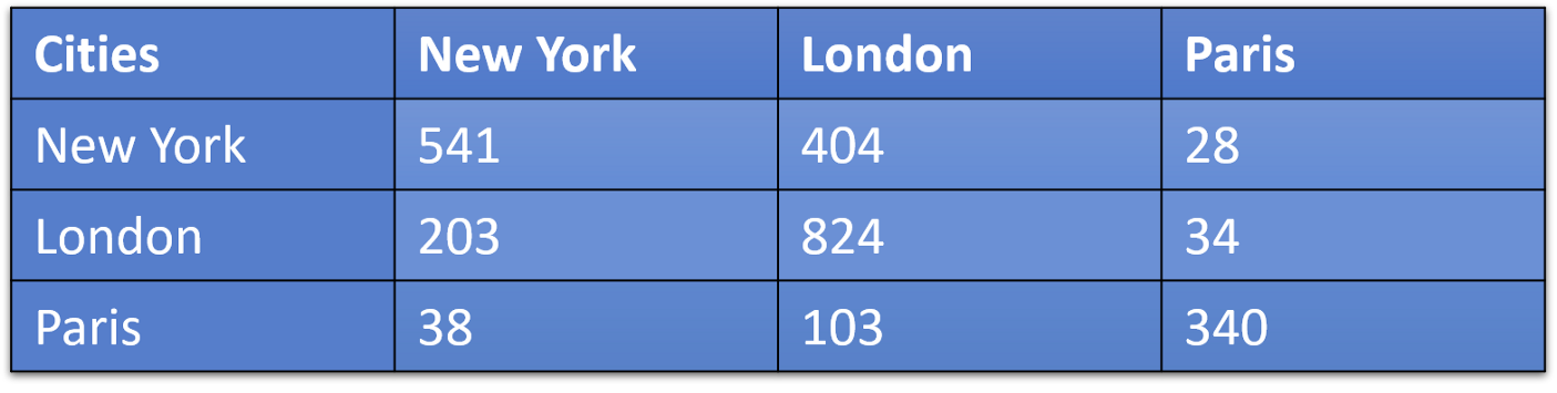
This can be interpreted as number of New York tweets that were classified as New York-541, London-404 and Paris-28.
Define a ADF (Augmented Dickey-Fuller) Test
The Dickey-Fuller test is one of the most popular statistical tests. It can be used to determine the presence of unit root in the series, and hence help us understand if the series is stationary or not. The null and alternate hypothesis of this test is:
Null Hypothesis: The series has a unit root (value of a =1) and is non stationary
Alternate Hypothesis: The series has no unit root.
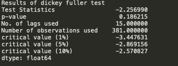
We see that the p-value 0.18 is greater than 0.05 so we cannot reject the Null hypothesis. Also, the test statistics is greater than the critical values. so the data is non-stationary and the null hypothesis is right.
To get a stationary series, we need to eliminate the trend and seasonality from the series. Remember that for time series forecasting, a series needs to be stationary. The series should have a constant mean, variance, and covariance. We need to take care of the seasonality in the series. One such method for this task is differencing. Differencing is a method of transforming a time series dataset. In order to perform a time series analysis, we may need to separate systematic seasonality and trend from our series (and one non-systematic component called noise). The resultant series will become stationary through this process.

See the data in your Google Account and choose what activity is saved to personalize your Google experience.
LikeLike
Nothing really exciting to see here, we have more occurrences of +/-4% days but that’s because we have more days, the overall distribution (and therefore the likelihood of that happening on a given day) has not changed.
LikeLike
But an important distinction here is that I said random days of extreme deviation. Look again at the real-world examples, the extreme days aren’t sprinkled throughout randomly, they’re clustered. This clustering makes sense, we can point to those three main clusters and say “dot-com bubble boom/bust,” “global financial crisis,” and “COVID-19.” Pick a stock and you can explain a period of volatility on a smaller scale as well.
LikeLike
What we have observed above, volatility is clustered.
Mandelbrot explains that traders intuitively understand that time in financial markets is relative; the first 15 minutes or the last 15 minutes of a given day’s market hours are generally more volatile, and on larger scales, days and weeks may seem this way. In fact, professional traders often speak of “fast” or “slow” markets. Due to this, he postulated the existence of “trading time” distinct from clock/calendar time.
LikeLike
The Markov property expresses the fact that at a given time step and knowing the current state, we won’t get any additional information about the future by gathering information about the past.
Die Markov-Eigenschaft drückt die Tatsache aus, dass wir zu einem bestimmten Zeitpunkt und bei Kenntnis des aktuellen Status keine zusätzlichen Informationen über die Zukunft erhalten, indem wir Informationen über die Vergangenheit sammeln.
LikeLike
Non-stationary data, as a rule, are unpredictable and cannot be modeled or forecasted. The results obtained by using non-stationary time series may be spurious in that they may indicate a relationship between two variables where one does not exist. In order to receive consistent, reliable results, the non-stationary data needs to be transformed into stationary data. In contrast to the non-stationary process that has a variable variance and a mean that does not remain near, or returns to a long-run mean over time, the stationary process reverts around a constant long-term mean and has a constant variance independent of time.
https://www.investopedia.com/articles/trading/07/stationary.asp
LikeLike
A random walk with or without a drift can be transformed to a stationary process by differencing (subtracting Yt-1 from Yt, taking the difference Yt – Yt-1) correspondingly to Yt – Yt-1 = εt or Yt – Yt-1 = α + εt and then the process becomes difference-stationary. The disadvantage of differencing is that the process loses one observation each time the difference is taken.
LikeLike
There isn’t any obvious non-stationary: the mean doesn’t seem time-varying, nor does the auto-covariance function, although the latter is harder to inspect visually. We can also do an augmented Dickey Fuller test, with the alternate hypothesis of no unit root (a unit root would imply non-stationarity).
adf.test(diff(data))
Augmented Dickey-Fuller Test
data: diff(data)
Dickey-Fuller = -4.4101, Lag order = 5, p-value = 0.01
alternative hypothesis: stationary
Thus we reject the null hypothesis of a unit root.
LikeLike
Statistical stationarity: A stationary time series is one whose statistical properties such as mean, variance, autocorrelation, etc. are all constant over time. Most statistical forecasting methods are based on the assumption that the time series can be rendered approximately stationary (i.e., “stationarized”) through the use of mathematical transformations. A stationarized series is relatively easy to predict: you simply predict that its statistical properties will be the same in the future as they have been in the past! (Recall our famous forecasting quotes.) The predictions for the stationarized series can then be “untransformed,” by reversing whatever mathematical transformations were previously used, to obtain predictions for the original series. (The details are normally taken care of by your software.) Thus, finding the sequence of transformations needed to stationarize a time series often provides important clues in the search for an appropriate forecasting model. Stationarizing a time series through differencing (where needed) is an important part of the process of fitting an ARIMA model, as discussed in the ARIMA pages of these notes.
Another reason for trying to stationarize a time series is to be able to obtain meaningful sample statistics such as means, variances, and correlations with other variables. Such statistics are useful as descriptors of future behavior only if the series is stationary. For example, if the series is consistently increasing over time, the sample mean and variance will grow with the size of the sample, and they will always underestimate the mean and variance in future periods. And if the mean and variance of a series are not well-defined, then neither are its correlations with other variables. For this reason you should be cautious about trying to extrapolate regression models fitted to nonstationary data.
LikeLike
Autocorrelation doesn’t cause non-stationarity. Non-stationarity doesn’t require autocorrelation. I won’t say they’re not related, but they’re not related the way you stated.
For instance, AR(1) process is autocorrelated, but it’s stationary:
LikeLike
Best Introduction to ARIMA:
https://www.machinelearningplus.com/time-series/arima-model-time-series-forecasting-python/
LikeLike
adf_test(train[‘#Passengers’])
– Strict Stationary: A strict stationary series satisfies the mathematical definition of a stationary process. For a strict stationary series, the mean, variance and covariance are not the function of time. The aim is to convert a non-stationary series into a strict stationary series for making predictions.
– Trend Stationary: A series that has no unit root but exhibits a trend is referred to as a trend stationary series. Once the trend is removed, the resulting series will be strict stationary. The KPSS test classifies a series as stationary on the absence of unit root. This means that the series can be strict stationary or trend stationary.
– Difference Stationary: A time series that can be made strict stationary by differencing falls under difference stationary. ADF test is also known as a difference stationarity test.
LikeLike
The lag drop-off for the partial autocorrelation function will be used to determine the AR term, while the lag drop-off for the autocorrelation function on the differenced series is used to determine the MA term in ARMA.
LikeLike
Normally in an ARIMA model, we make use of either the AR term or the MA term. We use both of these terms only on rare occasions. We use the ACF plot to decide which one of these terms we would use for our time series
If there is a Positive autocorrelation at lag 1 then we use the AR model
If there is a Negative autocorrelation at lag 1 then we use the MA model
LikeLike
You can test the model:
https://github.com/maxkleiner/maXbox4/blob/master/ARIMA_Predictor21.ipynb
LikeLike